
WASH Research & Development Centre · University of KwaZulu-Natal
A Standardised De-Risking Protocol for Water Efficient Sanitation Systems (WESS/NSS)
The reference model, the decision-tree activity set, the field diagnostics with their thresholds and decisions, the laboratory interpretation, the mitigation catalogue, and the live financial rating — a companion volume to The Water Efficient Sanitation Systems (WESS/NSS) Industry
A site is de-risked when
its configuration is declared against the WESS reference model, its risks are recorded in a live HAZOP register, its low-cost soft sensors stream data to a central platform, that stream shows the unit operating within its expected norms, and the staff who run it have been trained to keep it there. Version 6 adds the remaining step: the stream no longer produces a dated certificate but a continuously-computed rating that a lender holds as a covenant.
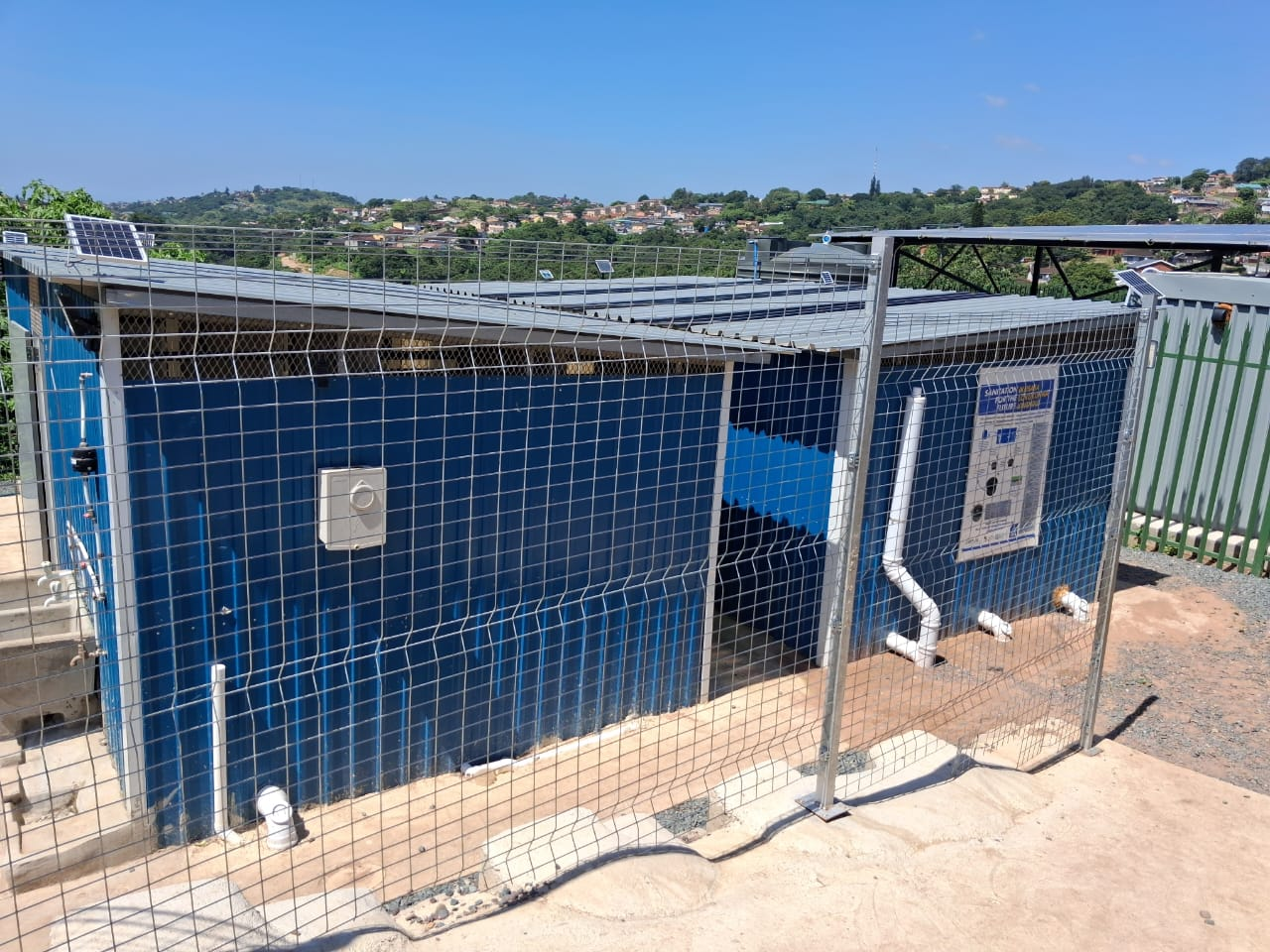
Timeframe & acknowledgement
This protocol was built and corrected over roughly 18 months of field work — the site visits, the diagnostics, the laboratory rounds and the reports that turned a design-time method into a field-tested one. It exists because the WESS technology providers — Enviroloo, Prana Aquonic, WEC and Lilliput — opened their installations to independent assessment and acted on the findings visit after visit. The evidence in this document is theirs as much as ours; the Centre's role was to measure, structure and de-risk what they built.
The WESS industry and the de-risking problem
Water Efficient Sanitation Systems treat waste at or near the point it is generated and recover the treated water for flushing or reuse — a workable way to extend sanitation into the peri-urban and rural settings that waterborne sewerage cannot reach at the required pace.
The state of sanitation, and where WESS stands
South Africa carries a sanitation backlog that conventional waterborne sewerage cannot close at the required pace: millions of households in dense peri-urban settlements and dispersed rural communities sit beyond the practical reach of trunk sewers and centralised treatment works, and the water those works would demand is itself under stress. Non-sewered sanitation is therefore not a stop-gap but a permanent category of infrastructure, and WESS — the sub-category that treats on site and recovers the water — is the form of it that answers the water constraint as well as the sewerage one.
The regulatory and standards ground has been prepared. ISO 30500 was revised in 2025 and sets the effluent and pathogen performance a non-sewered system must meet; ISO 31800 governs the treatment of the faecal-sludge stream; SANS 241 bounds any water that could reach human contact; and a draft framework for model by-laws now defines WESS as a category of non-sewered sanitation that may treat and reuse water on site without a water-use licence. On the piloting side, the engineering field-testing guidelines developed at UKZN and published with the International Water Association set out how a novel sanitation technology is taken through structured field trials. This protocol picks up where those guidelines end: piloting establishes that a technology can work; what follows here is the standardised troubleshooting and optimisation of technologies operating in the field — the stage of the innovation value chain between a successful pilot and a bankable, scaled deployment.
The work reported here was done to improve the industry and to build it towards providing high-quality technologies. The protocol serves the technology developers directly: every diagnostic that locates a failure mode is also a design input, and the providers assessed in this programme have acted on the findings visit after visit, so the assessment loop is simultaneously a product-improvement loop.
Standardising the skills as well as the tests
A protocol standardises more than measurements — it standardises the people. The sector is converging, in a discussion now running internationally, on a tiered skills ladder for non-sewered sanitation: the janitor, who keeps the facility clean and reports what a user sees; the operator, who runs the daily checks and the routine interventions; the technician, who executes the diagnostics in this document and acts on their decisions; and the advanced technician, who reads the laboratory results, maintains the HAZOP register and manages the mitigations. Each part of this protocol is written so that it converts directly into training material at the appropriate tier, under any of the three operating and maintenance arrangements a municipality may choose: O&M carried in-house by the municipality, O&M outsourced to sanitation service providers, or maintenance carried by the technology suppliers on their own installed base. The same tests, thresholds and decisions hold in all three; only the badge on the overalls changes.
The de-risking problem
The technology has been developed and deployed. Adoption has nonetheless been limited, and the limiting factor is the shortage of independent, site-level evidence that an installed unit performs to specification under real operating conditions.
The shortage has a technical side, a financial side, and a social side. Technically, a unit that meets its design criteria on commissioning day drifts from them over the following weeks as loading, temperature, power supply and maintenance vary; without structured monitoring the drift goes undetected until the recirculated water at the toilet interface has discoloured or begun to smell — at which point the user, not the engineer, discovers the failure. Financially, a provider seeking loan finance to deploy at scale meets a lender who has no independent operating record to price against, and who therefore prices the risk conservatively into the spread. Socially, the influent itself is a behavioural variable: what a household flushes, cleans with and diverts into the system drives the variability of the blackwater and greywater the unit must treat, so the de-risking of a site is inseparable from the overall operating and maintenance arrangement — the user practices, the cleaning-agent inputs and the demand pattern are part of the load case, not background noise.
De-risking, in the sense used here, is the conversion of a site from that state of uncertainty to a state of documented, monitored and managed risk — and, in v6, the maintenance of that state as a live, financeable signal.
The field programme and its reach
The team has assessed eight sites operated by four technology providers in KwaZulu-Natal and Gauteng, and issued six formal site reports — five baseline assessments and one mid-point review — with three further sites onboarded for first visits in Q3 2026. Across those assessments the team opened twenty-four HAZOP entries and raised forty-nine engineering recommendations, each traceable to a field measurement.
| Site | Provider | Visits issued | HAZOPs | Recs |
|---|---|---|---|---|
| Pholani Enviroloo | Enviroloo | Baseline + Mid-point | 6 | 17 |
| Ekuthuleni Shellcross | Prana Aquonic | Baseline | 4 | 6 |
| Oakford | Prana Aquonic | Baseline | 2 | 4 |
| Portion 80 Nooitgedacht | Prana Aquonic | Baseline | 7 | 11 |
| Upper Malacca (NEWgen) | WEC | Baseline + greywater | 5 | 11 |
| Catoridge · Inchanga · Lilliput HQ | Lilliput | Scheduled Q3 2026 | — | — |
The same eight diagnostics, seven completion criteria and HAZOP procedure held from a single household unit to the 620-household community system. The next parts explain why, and exactly how the assessment is carried out.
The WESS reference model — the gold standard
A WESS unit is not a fixed product. The same treatment functions recur in different combinations and at different capacities. The protocol treats them as one object by defining a single comprehensive reference model — the gold standard — and expressing every real unit as a configuration against it.
The model is a graph. Its nodes are the complete set of treatment functions a WESS unit can perform. An implementation — a technology case, or a specific installed site — is a subgraph: the nodes it instantiates, the edges that route flow between them, and the capacity weights those nodes and edges carry (design flow, working volume, population-equivalent). Two units with the same topology but different capacities are different weighted subgraphs; a unit that omits a whole treatment line simply drops those nodes.
De-risking begins by placing the site on this model. Once the site's subgraph is declared, everything downstream attaches to it: the diagnostics interrogate node types, the criteria roll up defined nodes, each HAZOP entry maps to a model node, and each criterion's live rating attaches to the nodes that produce its evidence.
Nodes carry options; capacities carry load
A node names a function; the technology that fills it is a choice the implementation declares. The disinfection node may be filled by chlorination, UV, ozonation or electro-disinfection — a chemical-free option that generates oxidants (hydroxyl radicals, ozone, hydrogen peroxide and chlorine species) in situ from electrical energy, and suits a decentralised, real-time-monitored unit because it needs no dosing supply chain and is electrically observable. The capacity weights are load-bearing: the weight on the greywater product edge is the design-versus-delivered yield criterion C7 measures — the field found a unit meeting quality at a tenth of design flow, on the graph a product edge whose weight had collapsed while upstream node statuses stayed green.
| Cohort implementation | Configuration (nodes present) | Capacity weight |
|---|---|---|
| Household unit (Enviroloo) | Blackwater line → disinfection → recirculation; no greywater line | single household |
| Portion 80 community system | Full blackwater line → disinfection → recirculation to head tanks; solar | 620 households |
| Upper Malacca (NEWgen) | Blackwater line and full greywater line (UF / ion-exchange) → disinfection | site-scale, two lines |
Because a diagnostic interrogates a node type rather than a product, the palette that assesses a household settling node assesses a community settling node; only the capacity weight differs. That is why the protocol held across scales — and why a new technology is onboarded by declaring its subgraph, not by writing a new protocol.
The decision model & the de-risking decision tree
Underneath the diagnostics, the criteria, the HAZOP register and the financial case sits a single decision model, and it is the organising thread of the whole protocol rather than one component among many.
The model has four steps, repeated across every compartment and every failure mode of a unit. A diagnostic produces a small set of measured signals. The signals combine into a functional index for the compartment they describe. The index is classified on a green / amber / red traffic-light. And each band carries a defined corrective intervention:
| Band | Meaning | The move |
|---|---|---|
| Green | Within norms | Continue and monitor |
| Amber | Drifting; early warning | An action taken before performance is lost |
| Red | Out of specification | A confirmatory test and an operational intervention |
Because every part of the engagement resolves to the same green/amber/red statement, the parts compose rather than sit side by side: each field diagnostic expresses the model through its own functional index; the seven criteria are the roll-up of those compartment classifications to the level of the unit; the HAZOP register is the same model viewed from the risk side (a deviation scored on the 5×5 matrix, the score setting the action's priority exactly as a traffic-light band does); and the v6 live rating is this same model made continuous. The design is drawn most directly from the microbial Functional Microbial Health Index, where six functional signals combine into one traffic-light for a compartment — v4 generalised that to the whole palette. Stating it explicitly is what lets a field assessment end in a decision and a next step at each compartment, not a table of numbers requiring expert interpretation after the visit.
The activity set — seven phases, seventeen steps
The engagement is executed as a structured diagnostic algorithm: seventeen steps across seven phases, each step specifying the test to perform, the criteria to evaluate, the branch to follow on the result, and the HAZOP entry it generates. The structure is branching, not linear — results at each step decide whether the assessment proceeds, branches to a root-cause investigation, or triggers a corrective action. This is the answer to "do we even enter this area?": a healthy upstream result closes the deeper branch and moves on; a failing one opens it. The algorithm is run at every visit and feeds directly into the HAZOP register in InfraTrack.
| Phase | Steps | Protocol | Focus |
|---|---|---|---|
| 1 · Settling | 1–4 | Protocol 1 | Compartment functionality, SVI/DSVI, root cause |
| 2 · Hydraulics | 5 | Protocol 2 | Residence time, dead volume, mixing |
| 3 · Sludge management | 6 | Protocol 3 | Blanket depth, accumulation rate, desludging |
| 4 · Biological | 7–10 | Protocol 4 | DO distribution, colour gradient, microbial health |
| 5 · Water quality | 11–12 | Protocol 5 | TDS, turbidity, colour, reboot assessment |
| 6 · Disinfection | 13–15 | Protocol 6 | Colour, odour, chlorine, E. coli |
| 7 · Site readiness | 16–17 | Cross-cutting | Consumables, sensors, power, HAZOP compilation |
The master decision tree below shows the gating between phases: the main spine is the pass path; a tripped gate branches right to a root-cause or mitigation action before the assessment continues.
Cross-reference matrix — step, parameters, thresholds, guide words
| Step | Parameters | Key thresholds | HAZOP guide words |
|---|---|---|---|
| 1 | Settled solids, clarity gradient | Progressive C1→C5 | No differentiation; partial failure |
| 2 | SV30, MLSS, SVI | SVI <120 good · 120–150 mod · >150 poor | Poor settleability; settling failure |
| 3 | Diluted SV30, TSS, DSVI | DSVI <120 recoverable · >150 intrinsic | High solids; biomass dispersal |
| 4 | DO (all zones), foam, cleaning products | DO <0.5 in anoxic/anaerobic | Over-aeration; surfactant; toxic inhibition |
| 5 | τ, HRT, τ/HRT, N (tanks-in-series) | τ/HRT >0.9 adequate · <0.7 severe | Dead volume; short-circuiting; poor baffling |
| 6 | Blanket depth, ratio, interface | <30% normal · 40–50 warn · >50 critical | Elevated blanket; desludging overdue |
| 7 | DO (aerobic, anoxic, anaerobic) | Aerobic 2–4 · anoxic <0.5 · anaerobic ≈0 | Insufficient aeration; zoning failure |
| 8 | Mixed-liquor colour by zone | Progressive lightening | No gradient; treatment ineffective |
| 9 | Froth (aerobic), gas (anaerobic) | Tan 2–5 cm froth; fine bubbles | Filamentous; surfactant; inactive community |
| 10 | Convergence of steps 2/3, 8, 9 | Multiple negative indicators | Community failure; reboot required |
| 11 | TDS, EC, turbidity, colour, pH | Colour ≤30 Pt-Co; TDS trend stable | Accumulation; colour non-compliance |
| 12 | Water level, consumption | Level stable; TDS within threshold | Water loss; reboot required; demand mgmt |
| 13 | Colour, odour, clarity at interface | Clear, odourless, slight residual | Treatment failure; excessive dosing |
| 14 | Free chlorine (DPD) | 0.2–0.5 mg/L | Insufficient/excessive Cl₂; recirc risk |
| 15 | E. coli (lab enumeration) | Below threshold with adequate Cl₂ | Particulate shielding; disinfection failure |
| 16 | Consumables, sensors, power, structure | All available & operational | Supply / power / structural risk |
| 17 | Compiled HAZOP register | 5×5 risk matrix scored | All guide words from steps 1–16 |
The three-visit engagement
Each site engagement is one three-visit cycle over twelve to sixteen weeks, the visits spaced to give the provider at least three weeks to act between them. The provider takes part in the assessment and responds to each report before the next visit.
Baseline
Declare the site's subgraph, run the observational diagnostics, open the HAZOP register, survey for sensor placement, install the sensors, take the first laboratory round and set the sampling schedule. V1 is a coverage floor, not a complete diagnosis.
Mid-point review
Run the full equipment-intensive diagnostic set — tracer, settling/TSS, disinfection — and the laboratory campaign, and verify the provider's first revisions.
Final assessment
Verify the provider's revisions, commission and validate the sensor stream against the criteria, and bring the site to its de-risked state and its opening rating.
The eight field diagnostics — full detail
Each diagnostic attaches to a node type, resolves its measurements into a functional index and a green/amber/red status, and carries its own branch logic — the test, the thresholds, the decision, and the mitigation. The step numbers refer to the decision tree in Part III. Every numeric cut-point in this part is an operational trigger — illustrative and under calibration against the field data and the surrogate-validation work; they encode the right direction of a decision, not a validated limit. The authoritative compliance numbers are the ISO 30500 values in Part VII. Microbial functional profiling (Protocol 8) is placed second, immediately after settling — it runs as the integrated Protocol 8 but is the diagnostic most directly tied to the unit's public-health purpose, so it leads rather than trails the palette. Open the protocol you need.
Sampling stations, method and cadence
Every diagnostic in this part rests on the same sampling discipline, stated once here. Where: each compartment is sampled at its outlet (the water leaving it carries the verdict on that compartment's function), with the influent, the recirculation or head tank, and the final product line sampled in the same round, so the train reads as a progression rather than a set of disconnected points; sludge samples are drawn from the compartment floor by sludge sampler at the same stations. How: samples are taken with the unit in normal use, not after a quiet period — a steady-state reading of an unloaded unit de-risks nothing; grab samples are taken mid-depth away from walls and inlets, in containers matched to the analysis (sterile for microbial, acid-washed for metals, zero-headspace for DO-sensitive determinands); field parameters (pH, EC, DO, ORP, temperature, turbidity) are read on site at the moment of sampling, because they do not survive transport; laboratory samples are coded against the chain-of-custody legend (Part VII), cooled, and delivered within the laboratory's holding times. When: the same stations are sampled at every visit, so visit-to-visit trends are like-for-like — the comparison, not the single value, is the diagnostic.
P1Compartment settling testSteps 1–4 · SVI / DSVI
Purpose
Evaluate the primary treatment function. A properly functioning compartment train produces a progressive improvement in supernatant clarity from compartment 1 through 5; deviations locate the failure.
Procedure
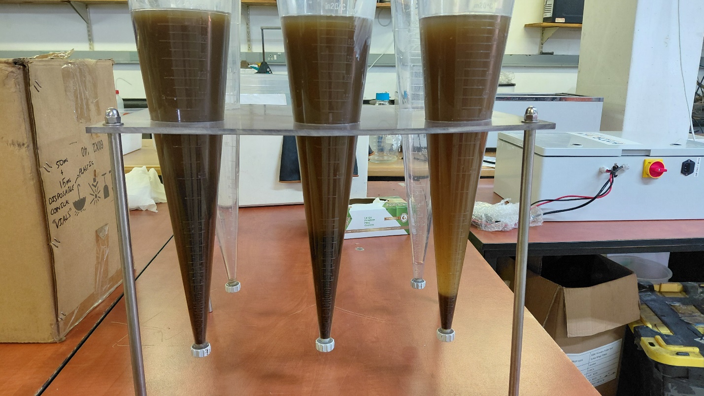
Collect 3 samples from each of the 5 compartments (15 total), settle in Imhoff cones for 30 min, and read the gradient. On the primary settler measure SV30 (mL/L at 30 min); with MLSS known, SVI = SV30 / MLSS. Where SV30 saturates the vessel, dilute iteratively until settled volume falls to 150–250 mL/L and compute DSVI = settled volume / TSS of the diluted sample.
Decision — SVI Step 2
| Reading | Classification | Decision |
|---|---|---|
| SVI < 120 mL/g | Good settleability | → Step 5 (hydraulics) |
| 120–150 mL/g | Moderate | Monitor → Step 5 |
| > 150 mL/g / no settling | Poor / failure | → Step 3 (DSVI) |
Decision — DSVI Step 3
| Reading | Classification | Decision |
|---|---|---|
| DSVI < 120 | Recoverable at lower conc.; high solids | Assess desludging → Step 5 |
| 120–150 | Moderate; investigate | → Step 4 (root cause) |
| > 150 / undetermined | Intrinsic biological/chemical problem; biomass dispersed | → Step 4 (root cause) |
Root cause & mitigation Step 4
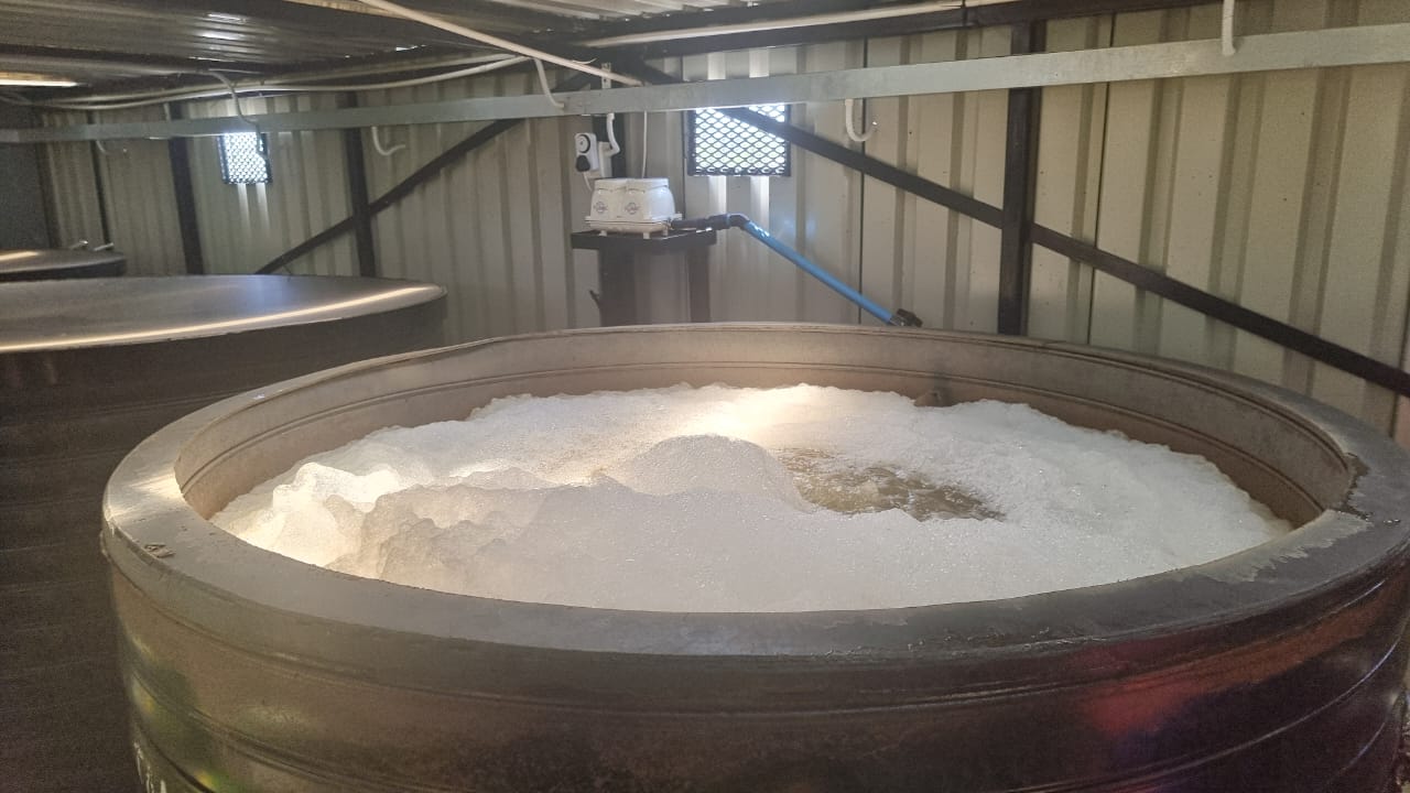
- DO > 2 mg/L in an anoxic/anaerobic zone → over-aeration, process zoning collapsed → reduce aeration rate, check baffle integrity. HAZOP: over-aeration.
- Foaming present → surfactant interference → identify cleaning products, community education on WESS-compatible products. HAZOP: surfactant loading.
- No foaming → possible toxic inhibition or very low food-to-biomass ratio → check influent for toxics, assess F:M, increase sludge feed from the primary settler. HAZOP: toxic / substrate imbalance.
- In all settling-failure cases → recommend a system reboot (partial or full water replacement to flush accumulated inhibitors); assess whether live bacterial culture is available on site to recharge the community after reboot.
Field example
Where the biomass settled poorly, standard SVI saturated (≈1000 mL/L, vessel-filling); the diluted index recovered ≈171 mL/g, corroborated against a measured aerobic SVI of 177. The protocol now carries the DSVI with its defined saturation trigger.
P8Microbial functional profilingWESScheck BioProfile · FMHI
Microbial detection is its own dedicated channel, not an inference from the physical-chemical sensors (pH, EC, ORP do not carry a biological count). It has three tiers, an on-site six-strip functional screen, a set of ratio indices, a joint-pattern decision logic, and a camera-read scoring system. The per-strip chemistry is proprietary and patent-pending through UKZN InQubate; this edition describes what each strip reads and how the results drive decisions, not the enabling formulations.
Three-tier architecture
| Tier | Instrument | Role | Status |
|---|---|---|---|
| 1 · Accredited lab | ISO/IEC 17025 culture / qPCR / metagenomics | Gold-standard confirmation; calibrates the tiers below | In use |
| 2 · WESScheck BioProfile | Six-strip lateral-flow functional profiler, camera-chip readout | On-site field screen; the fingerprint the rating consumes at each visit | Concept & methodology done; not yet built |
| 3 · Ramsurran continuous sensing | DNA-sequence detection panels; then a solid-state in-unit indicator read by a camera chip | Molecular E. coli detection near-term; the online stream medium-term | Exploratory |
The process-based panel already in place
Operational today: the COD Treatment-Train Profile (CTTP), the Oxygen Distribution and Operational Oxygen-Utilisation Profiles (ODP, OOUP), ORP, pH, temperature, TSS/turbidity, ammonia, nitrate/nitrite and gas production — integrated by a Metabolic State Assessment (MSA: ORP+DO+pH) into the green/amber/red Functional Microbial Health Index (FMHI) per compartment. Microscopy and an ATP activity kit are not yet available and are on the timeline.
The six-strip BioProfile — what each strip reads
| Strip | Reads | Bearing on the unit |
|---|---|---|
| 1 | Viable faecal-indicator activity (E. coli-associated) | Public-health / disinfection verdict |
| 2 | Total viable microbial activity — the denominator all indices normalise to | Whether the biology is alive at all |
| 3 | Gram-negative dominance | Enteric-signature context for the safety read |
| 4 | Biofilm & fouling risk | Membrane and pipework protection |
| 5 | AMR-enzyme screening signal | Antimicrobial-resistance pressure flag |
| 6 | Nitrogen-removal function | Whether biological nitrogen removal is active |
The functional indices (all normalised to the ATP baseline)
| Index | Calculation | Feeds criterion |
|---|---|---|
| ATP Activity Index | 1 − (test/control), inverse LFA | Total viable-activity baseline (denominator) |
| Faecal Viability (FVI) | viability signal, background-subtracted | Public-health / disinfection (safety) |
| Gram-neg Dominance (GNDI) | (GN·LPS / ATP) × 100 | Enteric-signature context for safety |
| Biofilm Fouling (BFI) | (EPS / ATP) × 100 | Fouling / membrane-protection risk |
| AMR Enzyme Pressure (AEPI) | (β-lactamase / ATP) × 100 | AMR sub-indicator (flag) |
| N-Removal Function (NRFI) | nitrate-reducer signal vs nitrate burden | Nutrient-removal process criterion |
The joint-pattern decision logic
The read is the joint pattern, never a single strip. Each strip scored visually 0–4 (camera image-analysis converts colour/fluorescence intensity to the indices later); the six sum to a Total BioProfile score 0–24, banded Low (0–4), Moderate (5–10), High (11–16), Very high (17–24). The report states "functional bacterial profile detected," never "bacteria identified" — a screening output, not a compliance score; positives trigger laboratory confirmation.
| Combined pattern | Interpretation | Action |
|---|---|---|
| High ATP + CQD+ + high GNDI | Viable activity with faecal & Gram-negative signature | Elevated public-health risk → confirm by culture/qPCR |
| High ATP + CQD− + high EPS | Activity without faecal signature; high fouling risk | Inspect filters, pipes, surfaces; clean / adjust operation |
| High ATP + high β-lactamase | Active biomass with possible AMR pressure | Confirm by AMR culture / qPCR / metagenomics |
| Low ATP + high LPS | Residual Gram-negative debris / endotoxin, not live dominance | Do not call live dominance without viability confirmation |
| High nitrate + low reducer signal | Nitrogen-removal biology weak/inactive | Check oxygen, carbon source, retention time, redox |
| ATP low, all others low | Low microbial-risk profile at time of test | Continue routine monitoring; periodic reference check |
The camera-chip reader (the "robot")
The kit is read not by eye but by a fixed-geometry camera-chip / smartphone reader: under controlled lighting a consistent region-of-interest is imaged, and image analysis converts colour or fluorescence intensity to a numerical index against a calibration chart — the step that makes the strip semi-quantitative and, later, the same colour-to-signal principle the Ramsurran solid-state in-unit indicator makes continuous and online. So tiers 2 and 3 are one arc: the strip readout made permanent.
How it wires to the rating
Each index becomes a criterion's compliance probability pₖ only through calibration against the accredited lab, so the BioProfile plugs into the same hierarchical, prospective validation as the physicochemical model — its maturity is earned, not assumed. And the physicochemical soft-sensors supply microbial confidence: turbidity, residual chlorine and high salts are known strip interferences, so a high reading lowers the confidence term cₖ for the microbial criterion. One channel carries the signal; the other says whether to trust it.
The microbial decision path (the tree, applied)
The microbial diagnostic ends in a decision the same way every other phase does — its own branching surface:
- 1 · Gather the compartment signals — CTTP (COD across chambers), ODP/OOUP (DO), ORP, pH, nitrate/nitrite, turbidity/TSS, sludge, foam/gas, and the BioProfile fingerprint where run.
- 2 · Classify the metabolic state — the MSA combines ORP + DO + pH into the dominant pathway (aerobic / anoxic / anaerobic / strongly reducing).
- 3 · Read the combined pattern, not the parameter — the integrated diagnostic matrix (Part VII) maps the pattern to a single diagnosis (organic overload, fermentation, denitrification, sulfide risk, washout, bulking, EPS overproduction, inhibition, collapse).
- 4 · Roll up to the FMHI band — the eight indicators give one green/amber/red per compartment: green → continue monitoring · amber → increase monitoring + corrective action · red → immediate investigation and intervention.
- 5 · Confirm and escalate — any BioProfile positive or red FMHI triggers accredited-lab confirmation (culture/qPCR) against the ISO 30500 Table 5 pathogen targets; a confirmed red is a HAZOP entry and, in v6, a rating driver.
P2Residence-time distributionStep 5 · lithium tracer
Purpose & procedure
Determine how effectively each compartment's physical volume is used. A lithium-chloride pulse-injection test constructs the RTD curve, closed with a mass-balance verification; short-circuiting and dead volume reduce effective residence time regardless of biological health.
Decision — mean residence time τ against HRT
| Reading | Classification | Decision |
|---|---|---|
| τ/HRT > 0.9 | Full volume utilised | → Step 6 |
| 0.7–0.9 | 10–30% dead volume | Investigate sludge accumulation, baffle integrity. HAZOP: reduced effective volume. |
| < 0.7 | Severe short-circuiting (>30%) | Urgent investigation. HAZOP: hydraulic failure. |
Mixing — tanks-in-series N
N < 2 near-complete mixing, poor baffling (assess baffle condition/modification) · N = 2–5 moderate, acceptable for most zones · N > 5 good plug-flow approach, effective baffling. Residence-time was the least-executed diagnostic at baseline (0 of 5 sites) — it is scheduled to V2 once equipment is mobilised.
Why it matters beyond the diagnostic
The fitted tank number N is not just a hydraulics score — it is the hydraulic input to the process model. Coupling the RTD to a biokinetic model is what lets the model separate a hydraulic failure (flow deviating from design, so biology never gets contact time) from a biokinetic failure (the microbes genuinely cannot keep up) — two causes a grab sample cannot tell apart. See Process modeling at the end of this part.
P3Sludge profile assessmentStep 6 · sludge judge
Procedure
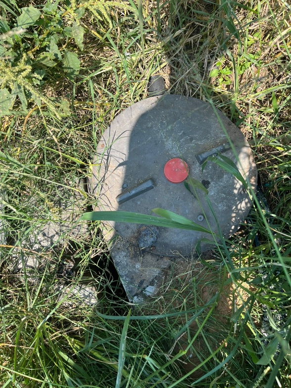
Deploy a Sludge Judge at each settling compartment, minimum 3 points (inlet, centre, outlet). Record sludge-blanket depth, total depth, interface quality, colour, consistency and gas bubbles. Blanket ratio = blanket depth as a percentage of total liquid depth.
Decision — blanket ratio
| Reading | Classification | Decision |
|---|---|---|
| < 30% | Within design limits | → Step 7 |
| 30–40% | Approaching limit | Monitor trend; HAZOP if trending upward |
| 40–50% | Warning | Schedule desludging. HAZOP: elevated sludge blanket. |
| > 50% | Critical | Desludge immediately. HAZOP: desludging overdue. |
Also record
Interface quality (sharp = normal compaction · diffuse = poor floc compaction, cross-reference Step 2). Spatial variation > 20 cm within a compartment → uneven flow distribution (HAZOP entry). Accumulation rate (V2/V3): if measured rate exceeds 1.5× design, raise a HAZOP entry for accelerated accumulation.
From a trend to a predicted threshold
Beyond the ratio bands, accumulation is quantified so a measured trend becomes a predicted threshold-crossing time: the rate is normalised per user (ΔV_sludge / (Δt · N_users)) and fed to a dynamic model — Stokes settling + a flocculation population-balance built for WESS's unstirred tanks + Kynch hindered settling + a tanks-in-series RTD. That model, and the risk-classification and valorisation decisions that follow from it, are set out in Sludge management & valorisation at the end of this part.
P4Biological activity assessmentSteps 7–10 · DO / colour / froth
Decision — DO distribution Step 7
| Zone / reading | Classification | Decision |
|---|---|---|
| Aerobic 2–4 mg/L | Adequate aeration | Continue |
| Aerobic < 1 mg/L | Insufficient aeration | Increase aeration / check blower-diffuser. HAZOP. |
| Aerobic > 4 mg/L | Excessive aeration | Reduce rate (floc breakage, energy waste) |
| Anoxic > 0.5 / anaerobic > 0.5 | Process zoning failure | Cross-reference Step 4 |
Colour gradient Step 8 & froth/gas Step 9
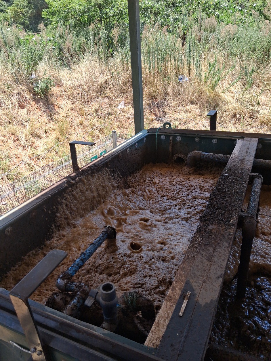
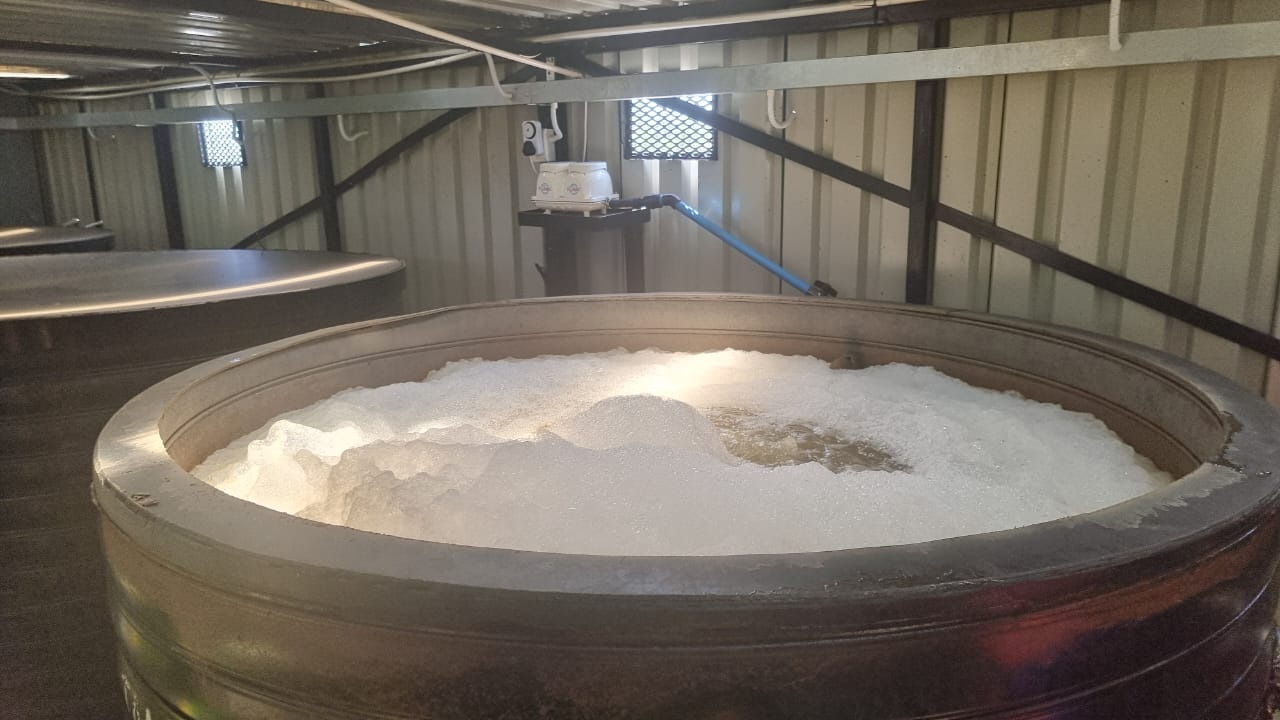
Colour: progressive lightening across zones = active treatment · minimal change = biological treatment ineffective. Aerobic froth: light, tan, easily dispersed (2–5 cm) = healthy · dense, dark, persistent = filamentous organisms or surfactant (cross-ref Step 4) · none = insufficient biomass. Anaerobic gas: steady fine bubbles = active methanogenesis · none = anaerobic community inactive.
Community failure & mitigation Step 10
When negative indicators converge — no colour gradient + no froth + no gas + poor settling (Step 2/3) — the biological community is absent or severely inhibited. Recommend: system reboot followed by reseeding with live bacterial culture. Investigate the die-off: toxic loading (check influent), chlorine recirculation (check disinfection–recirculation sequencing), extreme pH, or an extended power outage halting aeration. Flag: the site requires on-hand live culture for regular recharging — add to the O&M consumables list and procurement schedule.
Expectation bands per compartment illustrative · team-defined
The team maps each parameter to a Green (as designed), Amber (flag for next visit) and Red (immediate response) band per compartment type. The dominant ones:
| Aerobic (C4) | Green | Amber | Red → interpretation |
|---|---|---|---|
| DO (mg/L) | 2.0–4.0 | 1–2 or 4–6 | <1 or >6 — aeration failure / floc break-up |
| ORP (mV) | +50 to +200 | 0–50 or 200–300 | <0 or >300 — zoning collapsed |
| pH | 6.8–8.0 | 6.5–6.8 or 8–8.5 | <6.5 or >8.5 — acidification / ammonia toxicity |
| NH₄-N out | <3 | 3–10 | >10 — nitrification incomplete |
| SVI (mL/g) | 80–150 | 150–250 or 50–80 | >250 or <50 — bulking / pin-point flocs |
| Anoxic (C5) | Green | Amber | Red → interpretation |
|---|---|---|---|
| DO (mg/L) | <0.5 | 0.5–1.5 | >1.5 — O₂ carryover; denitrification stops |
| ORP (mV) | −50 to −100 | 0 to −50 or −100 to −150 | >0 or <−150 — zoning collapsed / fermentation |
| NO₃-N out | <5 | 5–15 | >15 — denitrification not delivering |
The complete 15-parameter × 10-compartment band matrix is a follow-up workshop deliverable for the engineering and microbial leads; the bands above are the operational subset in current use.
Leading indicator (v4)
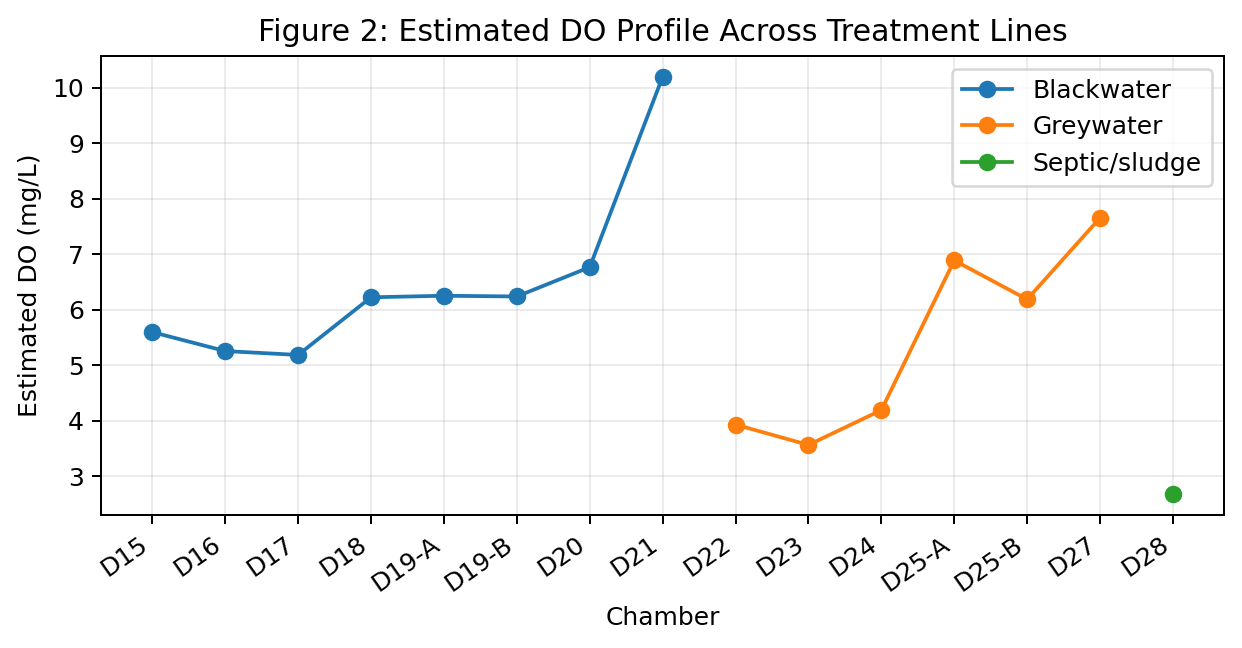
The V1 biological-activity DO profile — an anaerobic chamber reading aerobic-like DO — is a pre-registered leading indicator of later non-compliance on C1/C2. In the live rating it enters as a Watch (band B) trigger, not a breach.
P5Water concentration & rebootSteps 11–12 · TDS / colour
Purpose
Recirculating systems accumulate dissolved solids, colour and colloidal material over successive cycles. Measure TDS, turbidity, EC, colour (Pt-Co) and pH at the greywater compartment and recirculation tank; compare to the previous visit (or baseline at V1).
Decision — TDS trend Step 11
| Reading | Classification | Decision |
|---|---|---|
| Stable / decreasing | Mass balance managed | → Step 13 |
| < 5% / week | Slow accumulation | Monitor → Step 12 |
| 5–10% / week | Moderate | Assess reboot timing. HAZOP. |
| > 10% / week | Rapid | Reboot required soon. HAZOP. |
Colour & turbidity
Colour > 30 Pt-Co exceeds the ISO 30500:2025 limit → HAZOP: colour non-compliance. Turbidity rising while TDS stable = colloidal accumulation, polishing insufficient; both rising = general water-quality degradation.
Turbidity as the simpler field method. Where a Pt-Co colour comparison is not practical in the field, turbidity serves as the simpler routine surrogate: it is read in seconds on a hand-held meter (or by the same camera-under-fixed-lighting principle the protocol uses elsewhere), it trends with the colloidal and colour load in a recirculating system, and it is already a soft-sensor channel — so the operator tracks turbidity visit to visit and the Pt-Co measurement is reserved for confirming a suspected exceedance. The compliance value remains the Pt-Co number; turbidity is the trigger that says when to take it.
Reboot decision & mitigation Step 12
- Colour 30–50 Pt-Co → partial reboot (replace 30–50% of volume).
- Colour > 50 Pt-Co, or TDS above site threshold → full reboot (complete replacement).
- Flag: does the site have fresh water for reboot? If not → HAZOP: water supply for reboot not secured.
- Flag: excessive water use (continuous flushing)? If yes → HAZOP: water-demand management required.
P6Disinfection performanceSteps 13–15 · Cl₂ / E. coli
Interface sensory check Step 13
Clear, odourless, slight residual = adequate → confirm quantitatively · discoloured = upstream treatment failure (trace back through Steps 7–12) · septic odour = biological compartments underperforming · chemical odour = excessive dosing. The disinfection node's chosen technology (chlorination, UV, ozonation or electro-disinfection) must be placed and sequenced correctly in the recirculation loop; where electro-disinfection fills the node, its in-situ oxidant generation is directly observable in the ORP/residual stream.
Decision — free chlorine (DPD) Step 14
| Reading | Classification | Decision |
|---|---|---|
| 0.2–0.5 mg/L | Within target | → Step 15 |
| < 0.2 mg/L | Insufficient | Tablets exhausted → refill (HAZOP: Cl₂ supply); dosing blocked → clear; high upstream demand → cross-ref Step 11 |
| > 0.5 mg/L | Excessive; by-products, odour | Reduce dosing |
Design check: does chlorinated water recirculate through the biological zones? If yes → chlorine is suppressing the treatment bacteria → HAZOP: disinfection–recirculation sequencing (re-sequence the loop).
E. coli logic Step 15
Sample for laboratory enumeration (results at the next visit). Interpreting the returned value: below threshold with adequate Cl₂ = disinfection effective · elevated with adequate Cl₂ = particulate shielding, improve upstream treatment (cross-ref Step 11 turbidity) · elevated with no Cl₂ = complete disinfection failure (HAZOP).
Electro-disinfection — the node's chemical-free option
Where the disinfection node is filled by electro-disinfection, electrical energy generates the oxidants in situ — hydroxyl radicals, ozone, hydrogen peroxide and chlorine species — which attack the cell membranes, enzymes and genetic material of the pathogens that biological and physical treatment leave behind. It needs no dosing supply chain, suits a decentralised unit, and — the property that matters for de-risking — its whole state is electrically observable, so the disinfection node becomes one of the more readily streamed. Oxidant production is quantifiable by Faraday's law, which lets a lender-auditable set-point be derived rather than guessed:
So current and contact time set the oxidant dose, and the reading set that follows is the decision surface — each signal has a healthy target and a stress signature illustrative (set-points to be fixed against the unit and the ISO Table 5 pathogen targets):
| Signal | Healthy | Stress signature → action |
|---|---|---|
| E. coli / coliforms | Significant reduction / inactivation | Persistent presence or rising counts → confirm dose & contact time |
| ORP | In target oxidising range | Low / unstable / sudden drops → insufficient oxidant or high organic load |
| Residual oxidant (free Cl₂ / HOCl) | Maintained through contact period | Low / none → poor capacity or excessive demand → raise current / clean electrodes |
| Current density | Stable | Fluctuating / insufficient → reduced generation → check supply / cell |
| Voltage / cell potential | Within design range | Rising → electrode fouling / scaling → clean or replace electrodes |
| Conductivity | Sufficient for current flow | Low → weak electrochemistry → check salinity / cell |
| pH | ~ 6–8 (optimal for oxidant activity) | Too high/low → reduced inactivation → correct upstream |
| Turbidity / TSS | Low (oxidant contacts pathogens) | High → particulate shielding → improve upstream treatment |
| Energy consumption | Stable with effective removal | Rising with little gain → fouling / inefficiency |
| Electrode condition | Clean | Fouling / scaling / corrosion → maintenance |
Four of these signals — ORP, residual, current density and conductivity — are already SenseArray channels, so the electro-disinfection node streams its own health into the live rating and the HAZOP register in the same way the biological nodes do.
P7Greywater-stream performanceNEW in v4 · yield ≠ quality
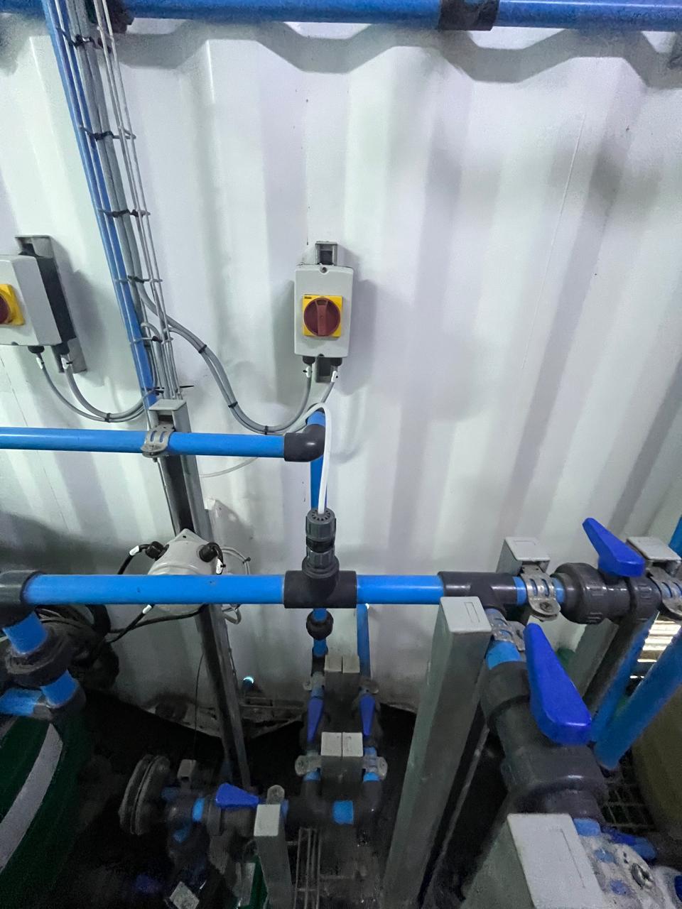
Added in v4 after the paired two-site greywater evaluation, which established that a mechanical greywater train (coagulation → ultrafiltration → ion-exchange/GAC → disinfection) can meet its quality target while delivering only about a tenth of design yield. The protocol separates the axes:
- Product-water yield against design — measured on a flow meter on the product line, now a protocol fixture (it is the capacity weight on the greywater product edge).
- UF integrity / membrane protection — a pressure-hold test with a trans-membrane-pressure log, since the recurring failure is the UF membrane fouled by upstream solids.
- Quality vs yield recorded separately — feeding the new completion criterion C7. A unit that treats correctly but delivers little recovered water is not de-risked on the recovery function.
Selecting the train — the greywater decision-support tool (Khanyinda)
The paragraph above de-risks a train that is already deployed. The prior question is which train to deploy, and no single technology is universally sufficient: physical steps remove solids but not dissolved organics; biological steps cut COD/BOD but suffer shock loading and surfactant inhibition; natural steps (constructed wetlands, soil filtration) polish but do not reliably hit microbial targets; chemical disinfection is the final barrier but its effectiveness depends on upstream turbidity and organic demand. The answer is a multi-barrier train — physical pre-treatment (screen + grease trap) → biological (biofiltration / MBBR) → natural polishing (constructed wetland / soil filtration) → chemical disinfection — with the specific units chosen from the influent characterisation.
The governing rule — BOD/COD ratio
Biodegradability decides whether biological treatment will even be efficient: BOD/COD = BOD₅ ÷ COD.
| BOD/COD ratio | Interpretation | Treatment implication |
|---|---|---|
| > 0.5 | Highly biodegradable | Biological treatment (NBS or engineered) will be efficient |
| 0.3–0.5 | Moderately biodegradable | Hybrid treatment system recommended |
| < 0.3 | Poor biodegradability | Chemical / advanced-oxidation pre-treatment |
Influent thresholds → pathway illustrative · team-defined
Each characterisation parameter is banded NBS-suitable / needs-attention / action-required — the same green/amber/red move the rest of the protocol uses, applied to greywater selection:
| Parameter | NBS suitable | Needs attention | Action required |
|---|---|---|---|
| Turbidity (NTU) | < 50 | 50–150 | > 150 → bio-treatment / pre-screening |
| TSS (mg/L) | < 100 | 100–250 | > 250 → settling required |
| pH | 6.5–8.5 | 5–6.5 / 8.5–10 | < 5 or > 10 → neutralisation |
| COD (mg/L) | < 150 | 150–500 | > 500 → engineered bio-treatment |
| BOD₅ (mg/L) | < 100 | 100–300 | > 300 → engineered bio-treatment |
| BOD/COD ratio | > 0.5 | 0.3–0.5 | < 0.3 → chemical pre-treatment |
| Total nitrogen (mg/L) | < 15 | 15–40 | > 40 → nutrient removal |
| Total phosphorus (mg/L) | < 5 | 5–20 | > 20 → nutrient removal |
| Oils & grease (mg/L) | < 20 | 20–50 | > 50 → grease trap required |
| Surfactants — MBAS (mg/L) | < 15 | 15–40 | > 40 → inhibits biological treatment |
| Electrical conductivity (mS/m) | < 70 | 70–200 | > 200 → dilution / desalination |
| E. coli (CFU/100 mL) | < 10 | 10–100 | > 100 → UV / chlorination disinfection |
Pathway logic
| Pathway | Trigger conditions | Representative systems |
|---|---|---|
| Nature-Based Solution (NBS) | COD < 300, TSS < 150, E. coli < 100, BOD/COD > 0.5 | Constructed wetlands, soil biofilters, green walls |
| Engineered bio-treatment | COD > 500, or BOD > 300, or turbidity > 200 | Membrane bioreactor (MBR), activated sludge, trickling filters |
| Hybrid system | Intermediate-strength; not meeting NBS criteria | Combination of physical, biological and disinfection units |
The reuse destination sets the target quality — differentiated, not uniform
The thresholds above characterise the influent; the treatment target is set by the destination, and one uniform quality for all reuse is the wrong specification — it over-treats some routes and under-protects others. The protocol therefore reads reuse against a differentiated ladder:
| Destination | Governing concern | Quality logic illustrative |
|---|---|---|
| Toilet flushing (closed loop) | User contact is incidental; aesthetics drive rejection | The ISO 30500 recirculated-water values govern — colour ≤ 30 Pt-Co, the pathogen log-reductions, and odour; the E. coli band above is set for incidental contact and aerosol exposure at the pan, which is why it is this strict for a water no one drinks |
| Fertigation (subsurface / drip to crops) | Pathogens and salts, not nutrients | Nitrogen and phosphorus are the benefit, not the contaminant — the TN/TP action bands invert, and the nutrient load is credited against fertiliser demand; the governing limits become the pathogen values (WHO reuse guidance; ISO 30500 Category B), EC/sodium for soil health, and boron/chloride for crop sensitivity |
| Surface irrigation & landscape | Contact and runoff | Pathogen limits tighten with public access; salinity and sodium-adsorption ratio govern long-term soil structure |
| Soakaway / managed infiltration | The receiving ground, not the water | Acceptability is a geotechnical and hydrogeological question — percolation, water-table depth, and whether the setting is water-sensitive; where the geotechnical analysis clears the site and water-sensitivity is not an issue, the water-quality bar is the lowest on the ladder |
Each site's reuse destination is declared at baseline, the applicable column of limits attaches to criterion C1, and a site that changes its destination (extending flush-water reuse to a garden, say) re-enters the ladder at the stricter row.
De-risking the greywater train — critical-indicators diagnostic
Once a pathway is selected and built, it is de-risked the same way as the rest of the unit — a staged verification (baseline → mid-point after each barrier → final log-reducible pathogen removal) reading the pattern across physical, organic, nutrient and microbial indicators, not one number:
| Observed condition | Likely diagnosis | Recommended check |
|---|---|---|
| High turbidity + high TSS | Excessive particulate / solids loading | Inspect pre-screening and settling capacity |
| Low BOD/COD (< 0.3) | Poor biodegradability | Chemical / advanced-oxidation pre-treatment |
| High COD/BOD, normal TSS | Dissolved organic load beyond biological capacity | Assess engineered bio-treatment (MBR, activated sludge) |
| High TN or TP | Nutrient loading from detergents / food waste | Add a nutrient-removal stage to the hybrid train |
| High surfactants (MBAS) | Detergent-driven inhibition of biology | Review household detergent use; consider pre-treatment |
| High EC | Salinity risk from softeners / certain detergents | Evaluate dilution or desalination needs |
| High E. coli despite good COD/TSS removal | Disinfection barrier failure or bypass | Verify UV/chlorination dosing and contact time |
| pH outside 5–10 | Household chemical contamination | Add neutralisation pre-treatment |
This greywater treatment-selection and de-risking work is led by Gloseje Khanyinda (greywater characterisation and treatment sequencing), and its experimental programme will turn these illustrative thresholds into validated ones across the cohort's sites.
Process modeling — the biokinetic model, coupled to RTD (Khan)
The diagnostics measure what a unit is doing now; a mechanistic process model predicts what it will do under conditions not yet seen — a load shock, an aeration failure, a new site's influent. WESS units resist prediction from design assumptions because they run under variable loading, intermittent flow and non-ideal hydraulics.
The model's central job in de-risking is to separate two failure modes a grab sample cannot distinguish: a biokinetic failure — the microbial community cannot degrade the load fast enough — and a hydraulic failure — the reactor's actual flow deviates from the ideal, so nominally adequate biology never gets adequate contact time. Coupling a biokinetic model to the residence-time distribution resolves the ambiguity, and is the core modeling contribution of this work.
The biokinetic model
Two mechanistic frameworks: ASM2d (19 state components — carbon oxidation, nitrification, denitrification and biological phosphorus removal) coupled with UCTADM1 (13 state variables, 10 reactions — anaerobic degradation of organic matter and methane production). State variables are linked by a stoichiometric Petersen matrix, each process rate a Monod, Contois or first-order expression. The general mass balance for a reactor element of volume V receiving flow Q:
Oxygen enters the aerobic switch through a transfer term kLa·(SO2,SAT − SO2), carried in the code as a dissolved-oxygen-saturation boundary so the switch responds to a realistic, time-varying oxygen field rather than a fixed input. The aeration coefficient kLa — not the saturation constant — is the physically meaningful lever the de-risking work fits. The balance above is written for the liquid phase only: the gas-phase transfer of CH₄/CO₂/H₂S that governs alkalinity, pH and methane on the anaerobic side is a required extension, not yet in the liquid-only form.
What runs today, and what is planned
This distinction is needed to read the indicator table below honestly. Implemented now: a reduced three-process matrix — hydrolysis, aerobic growth and lysis — that closes the full mass balance of COD, alkalinity and suspended solids and returns the carbon-and-solids state (SS, XS, XH). It is assembled from five core components — initial conditions, influent characterisation, oxygenation, stoichiometry and process kinetics — integrated through the reactor mass balance and solved sequentially in each TIS compartment, so transport, biological reaction and oxygen transfer resolve together. It does not yet resolve nitrogen, phosphorus or the anaerobic/methane pathway. Planned: the full ASM2d (nitrification, denitrification, biological-P) and UCTADM1 (anaerobic digestion, methane) that add the nitrogen, phosphorus, methane and VFA state. The indicator table further down is therefore the full-model target set; only its carbon-and-solids rows are live in the current reduced model, and the rest are marked planned.
The hydraulic coupling — Tanks-in-Series
The reactor is discretised into N ideally-mixed tanks in series (with a toggle to a single CSTR). The TIS residence-time distribution has a closed form:
As n → ∞ it sharpens toward ideal plug flow; at n = 1 it recovers the single-CSTR exponential decay. Fitting n from the tracer data (the P2 diagnostic) is a direct, physically interpretable measure of how far a reactor deviates from its design intent — and the hydraulic input the biokinetic model needs. Assuming ideal CSTR hydraulics would neglect that deviation and bias the biological prediction. The tracer is what makes the separation identifiable at all: from an effluent value alone the two failure modes are degenerate — a unit with capable biology but short-circuiting hydraulics, and one with adequate hydraulics but struggling biology, can return the same number — so pinning n independently from the tracer curve leaves the biokinetics as the only remaining unknown to fit.
De-risking the model — three stages
A calibrated model is trustworthy only once it has been shown to predict, not merely fit. So the model is de-risked with the same rigour as the physical unit, in three stages that mirror the three-visit engagement:
- Baseline — establish the stoichiometric matrix and kinetic parameter set, implement the mass balance and TIS configuration, and calibrate against baseline plant and tracer data.
- Mid-point — sensitivity analysis on the key parameters (μmax, KS, KO2, n, τ), fit a tank-indexed decay ki(t) to the field tracer curves, and evaluate residual-error trends.
- Final verification — confirm the model reproduces independent, out-of-calibration plant data, quantify parameter and prediction uncertainty, and document readiness for scenario-based de-risking of new WESS units.
Critical indicators — read together, never alone
Mass-balance closure error, effluent COD/N/P prediction error, biomass trends, sludge retention time, the tank number N fitted from tracer, and the agreement of the coupled model against the measured tracer curves. The interpretation is joint: a good biokinetic fit with a poor hydraulic fit (or vice versa) means the two sub-models are compensating for each other, not that both are correct. The full-model target set follows — only the carbon-and-solids rows are live in the current reduced model (see above); the rest are marked planned:
| Model prediction | Healthy | Stress signature |
|---|---|---|
| Readily biodegradable COD (SS) | Rapidly consumed by heterotrophs | Elevated → overloading or low biomass activity |
| Particulate organics (XS) | Gradual hydrolysis to substrate | Accumulation → hydrolysis rate-limiting / low solids retention |
| Heterotrophic biomass (XH) | Stable — supports COD removal & denitrification | Decay / washout → poor, unstable COD removal |
| Autotrophic biomass (XA) planned | Stable nitrifier population | Reduced → incomplete nitrification, high ammonia |
| Ammonium (NH₄⁺-N) planned | Falls through nitrification | Persistent → O₂ limitation, inhibition or overload |
| Nitrate/nitrite (NOₓ-N) planned | Produced then reduced | Accumulation → poor denitrification; low → nitrification failure |
| Orthophosphate (PO₄³⁻-P) planned | Reduced by biological P removal | Elevated → poor uptake or stressed PAO |
| Dissolved oxygen (DO) | Within target range | Low limits nitrification; high suppresses denitrification & wastes energy |
| Alkalinity | Consumed gradually, pH held | Excessive depletion → pH decline, inhibits nitrification |
| Methane (CH₄) planned | Stable generation → efficient digestion & COD conversion | Reduced → microbial inhibition, overload or poor digestion |
| Volatile fatty acids (VFAs) planned | Formed and consumed in balance | Accumulation → acid-vs-methanogen imbalance, digester instability |
| Biogas production planned | Stable yield → healthy anaerobic degradation | Declining → reduced microbial activity or inhibition |
| Anaerobic biomass planned | Stable → sustains hydrolysis, acidogenesis, acetogenesis, methanogenesis | Loss/inactivity → lower digestion efficiency & methane |
| COD removal efficiency | High (combined aerobic + anaerobic) | Reduced → overloading, inhibition or short retention |
| Sludge production | Stable → balanced microbial growth and decay | Excess or reduced biomass → process imbalance or washout |
| Effluent quality | Low COD, ammonia, nitrate, phosphate | Elevated → one or more biological processes deteriorating |
This process-modeling work is led by Muhammad Ameen Khan (process modelling and residence-time analysis), building the WESS process and population-balance models that the field diagnostics calibrate.
Sludge management & valorisation — the decision framework (Vundla)
A WESS unit can look healthy on inspection and still carry undetected risk in what settles at the bottom. WESS sludge is more concentrated, more variable and more pathogen-rich than conventional wastewater sludge, and no structured management framework exists for it in the South African context — a gap municipalities cite as a barrier to adopting WESS at all. This work builds the first evidence-based sludge-management decision framework for WESS, grounded in field data from four operational installations.
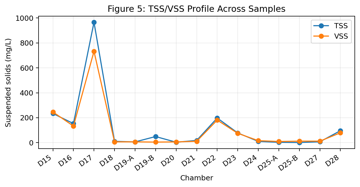
Preliminary sampling has already confirmed the scale of the problem: significant inter-site variability in solids and organic loading, consistently acidic conditions (pH low enough to point to unmanaged acidogenesis, to be confirmed against VFA), and pathogen loading above acceptable limits. A site anomaly — effluent TSS exceeding influent TSS at one site — is flagged for resampling rather than smoothed over.
Progress to date — an underway programme, not a proposal
The framework is being built on field data and a working model already in hand, not on a plan. What is banked:
| Activity | Status | Output |
|---|---|---|
| Site sampling & characterisation (Obj. 1) | Complete at 3 of 4 sites | Physicochemical results across sites — total solids, COD, pH, E. coli |
| Sludge-blanket height field monitoring (Obj. 2) | Ongoing — Week 5 data collected | Live workbook; condensed field report (Rev. 3), Upper & Lower Malacca, three tank types per site |
| Flocculation kinetics / PBE model (Obj. 2) | Kernel rebuilt for unstirred WESS; first run complete | Working Python implementation; documented seven-step procedure with equations |
| Settling-performance groundwork (Obj. 3) | SV30/DSVI batch data available | First-pass calibration input identified, not yet applied |
| Risk classification, techno-economic screening, framework integration (Obj. 4–7) | Not yet started | Dependent on Tours 2 & 3 and full characterisation |
The framework — a pipeline, not a set of sub-projects
Two questions organise the work: how sludge characteristics, accumulation rates and risks can be systematically characterised and classified, and how a techno-economic and risk-based rule set can link those classes to treatment and valorisation pathways. The pipeline: characterise across physical, chemical, biological and thermal properties → quantify how fast sludge accumulates → assess how well it settles → classify into risk classes → screen valorisation options against cost and feasibility → integrate into one decision tool for operators and planners.
Characterisation panel
| Domain | Parameters | What they inform |
|---|---|---|
| Physical | TS, VS, TSS, VSS, moisture, particle size, density, SVI/DSVI | Settleability & accumulation behaviour |
| Chemical | COD, SCOD, BOD₅, TKN, NH₃-N, TP, alkalinity, pH, conductivity, heavy metals | Treatment demand & valorisation suitability |
| Biological | E. coli, total coliforms, helminth ova, floc/filamentous microscopy (Eikelboom) | Pathogen risk & settleability failure modes |
| Thermal pending | Proximate + CHNS elemental analysis | Energy-recovery screening |
Accumulation — a population-balance model built for unstirred tanks
Blanket depth is measured with a Sludge Judge at three positions per tank across visits and converted to volumetric and volatile-solids accumulation rates (L/user·day, kgVS/user·day). Predicting the time to the desludging threshold needs a settling model, and here the standard approach breaks: WESS tanks are unstirred, so the shear-driven aggregation kernel of conventional settling models does not apply. The model instead tracks the full floc-size distribution n(L,t) through aggregation, breakage and settling loss:
The kernel is built from Brownian motion and differential settling; at the tens-to-hundreds-of-µm floc sizes of sludge, differential settling dominates and the Brownian term is essentially inactive. The one fitted parameter is the collision efficiency α. Collapsing the distribution into its moments gives two field-measurable outputs from instruments already in the panel, with no floc imaging required: TSS ∝ M₃ (floc volume) and turbidity ∝ M₂ (floc surface area). Because aggregation conserves floc volume but not surface area, the model predicts a clean diagnostic signature — turbidity falls faster than TSS during early aggregation — readable directly from a turbidimeter and a TSS measurement.
A first material-balance run (settling tank as a tanks-in-series reactor, N = 5) yields a predicted desludging-threshold time that is now being reconciled against the multi-week Sludge-Judge blanket series; that model-versus-field check is the validation step, and the accumulation rates it produces are the primary publishable output (Paper 1). Those rates do four jobs at once: they turn a measured blanket trend into a predicted threshold-crossing time for desludging scheduling, put every site on a common quantitative footing for cross-site comparison, feed the risk classification directly, and provide the field series the model is validated against.
Risk classification & valorisation decision rules
Sludge is classified into risk classes on pathogen loading, organic content and handling requirement; techno-economic rules then link measured characteristics to candidate pathways, converting a measured quantity directly into an operational decision:
- C:N ratio 20–40 with helminth ova present → composting candidate only with a thermophilic pasteurisation step to inactivate the ova before any land application.
- High biodegradable COD, low heavy-metal load → anaerobic-digestion candidate.
- High organic/carbon content, low moisture → pyrolysis candidate (added once thermal characterisation is available).
Risk is scored on likelihood and consequence: high-risk findings require immediate corrective action, medium risks monitoring and optimisation, low risks routine surveillance. A single favourable reading does not offset a disqualifying one — a high heavy-metal load restricts every pathway regardless of the rest.
Valorisation pathways under consideration
| Pathway | Principle | Best suited to |
|---|---|---|
| Anaerobic digestion | Biological breakdown of organic matter under anoxic conditions, producing biogas | High biodegradable COD, low heavy-metal load |
| Agricultural reuse | Land application after thermophilic pasteurisation to inactivate pathogens | Sludge within acceptable heavy-metal and pathogen limits post-treatment |
| Pyrolysis pending thermal data | Thermal decomposition in the absence of oxygen, producing biochar | High organic/carbon content, low moisture |
| Composting with pasteurisation gate | Aerobic biological stabilisation to a soil conditioner; thermophilic phase (or a separate pasteurisation step) inactivates pathogens including helminth ova | C:N ratio 20–40; bulking material available; land-application route open |
| Other thermal routes screening stage | Drying-plus-combustion (the LaDePa pattern), gasification, and hydrothermal carbonisation each trade moisture tolerance against energy input and product value | HTC where moisture is high; combustion/gasification where a heat or power sink exists; all gated by the same heavy-metal and emissions screens |
The pathway set is deliberately open — composting, biochar and the wider thermal family enter the comparison as their characterisation data arrives, and the techno-economic screening ranks whichever pathways the site's sludge qualifies for; the framework fixes the method of choosing, not a fixed menu.
Settling & accumulation as a diagnostic — read together
| Observed pattern | Condition | Operational meaning |
|---|---|---|
| Low SVI/DSVI, steady accumulation | Well-settling sludge | Routine monitoring; desludge as predicted |
| Rising SVI/DSVI, filamentous growth | Poor settleability developing | Investigate floc condition; review upstream loading |
| Accumulation diverging from model | Model–data mismatch | Re-examine site-specific settling / flocculation assumptions |
| High COD with high moisture | Low energy density | Reduces thermal-conversion suitability; consider AD or composting |
| E. coli / helminth ova above threshold post-treatment | Pathogen risk unresolved | Escalate risk class; reassess valorisation pathway |
De-risking the framework — three stages
- Baseline — full characterisation and initial accumulation/settling data across the four sites; already complete at three of four.
- Mid-point — accumulation modelling, risk classification, technology review and techno-economic screening; draft Paper 1.
- Final verification — integrate into the decision framework, validate against field data across all sites, submit Papers 1 and 2.
Objectives 4–7 (risk classification, techno-economic screening, framework integration) are not yet started; they depend on completing the remaining site tours and full characterisation. The framework stays site-conditional — the inter-site variability already observed means no single pathway suits all four sites.
This sludge-management framework is the MSc work of Mxolisi Vundla, supervised by Prof. Randhir Rawatlal and Dr. Samuel Tenaw Getahun, targeting two papers — Paper 1 (accumulation & characterisation; Water SA, target Q4 2026) and Paper 2 (risk-based decision framework; Journal of Environmental Management, target Q2 2027).
The seven completion criteria
Each criterion carries a status of Met, On track, At risk or Not yet assessed — the unit-level roll-up of the green/amber/red compartment classifications. They are tracked separately even where they correlate, because the dependence between them is what the diagnostic palette is designed to expose.
| Criterion | Definition | Evidence base |
|---|---|---|
| C1 Effluent quality | Laboratory parameters within compliance bands for the reuse destination | P6 + lab round; sensors at calibration (ISO 30500; SANS 241) |
| C2 Process integrity | Each compartment delivering its intended treatment function | Protocols 1–4 |
| C3 Infrastructure condition | Mechanical and structural fit for purpose | P3 + visual inspection + photographs |
| C4 Operator capability | Trained, equipped and registered against the HAZOP register | Training log + HAZOP |
| C5 Sensor coverage | Streaming and calibrated against at least two laboratory rounds | Sensor package; installed at V1 |
| C6 Social acceptance | Use without rejection, vandalism, misuse or community complaint | Social assessment |
| C7 Product-water yield | Delivered volume within tolerance of design output, where the unit recovers water | P7 product-line flow metering |
Tiered social framework: acceptance to capability (phase 2)
C6 records whether a community accepts the unit; C4 records whether its operators can run it. Between the two sits the behavioural ground the influent-variability finding (Part I) makes unavoidable, and phase 2 of the de-risking programme structures it as a tiered framework that shifts a site progressively up four rungs: awareness — the users know what the system is, what it recovers, and what must not enter it; education — the janitors and households understand why the rules hold (what a surfactant surge or a diverted greywater line does to the biology they depend on); behavioural nudges — the defaults, signage, dispenser choices and feedback that make the compliant behaviour the easy one, applied before enforcement is ever considered; and training — the formal ladder of Part I (janitor → operator → technician → advanced technician), with competence registered against the HAZOP register exactly as the engineering mitigations are. A site climbs the rungs in order, its position is recorded alongside C4 and C6 at each visit, and the aim is that by the final visit the social state of the site is as documented, monitored and managed as its process state — which is the definition of de-risked applied to people rather than to compartments.
Laboratory results & interpretation guide
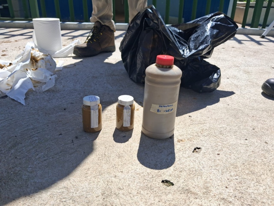
The sensor stream tracks parameters that correlate with performance but cannot directly measure every regulated indicator, so a structured laboratory schedule provides the definitive measurements. Three sampling events are conducted across the engagement, one per visit, aligned to ISO 30500:2025 and collected by trained engineers in sterile containers under chain-of-custody. This part sets out the compliance framework the results are read against, the decision each value drives, and the integrated diagnostic interpretation that turns a chamber-by-chamber data set into a single microbial diagnosis.
The compliance framework — ISO 30500:2025
ISO 30500:2018 was adopted as SANS 30500:2019; the second edition, ISO 30500:2025 (July 2025), updates the performance requirements, and the Centre sits on the SABS standards-writing division adapting it for South African conditions. A unit is first classified — Class 1/4 (backend non-biological) or Class 2/3 (backend includes one or more biological treatment processes), single- or multi-frontend — which sets its test route; this is the same declaration as placing the unit's subgraph on the reference model. The standard then fixes the numbers below. These are authoritative, not illustrative.
Environmental parameters ISO 30500 Table 6 — recirculated water & effluent
| Parameter | Category A — unrestricted urban reuse | Category B — restricted reuse / discharge to surface water |
|---|---|---|
| COD | ≤ 50 mg/L | ≤ 150 mg/L |
| TSS | ≤ 10 mg/L | ≤ 30 mg/L |
| BOD₅ | ≤ 10 mg/L | ≤ 30 mg/L |
Nutrients Table 7 · pH & colour Table 8
| Parameter | Requirement (meet either) |
|---|---|
| Total nitrogen | ≥ 70% load reduction OR ≤ 15 mg/L |
| Total phosphorus | ≥ 80% load reduction OR ≤ 2 mg/L |
| pH | 6.0 to 9.0 (all reuse) |
| Colour | ≤ 30 Pt-Co (recirculated water only) |
Human-health — max concentration & log-reduction Table 5 (liquid)
| Pathogen class | Surrogate / indicator | Max in liquid | Overall LRV |
|---|---|---|---|
| Bacterial | E. coli | ≤ 100 /L | ≥ 6 |
| Viral | MS2 coliphage | ≤ 10 /L | ≥ 7 |
| Helminth | Ascaris suum ova | < 1 /L | ≥ 4 |
| Protozoa | Clostridium perfringens spores | < 1 /L | ≥ 6 |
Noise must not exceed 60 dBA (LEX,24h) and never 85 dBA (LpA,max); odour reported as unpleasant-or-unacceptable must stay ≤ 10% of observations (≤ 2% "unacceptable"). Where recirculated water may be ingested (hand-washing, anal cleansing) the Table 5 pathogen log-removal applies with physical barriers and signage; for reuse (e.g. irrigation) the DWS Revised General Authorisations (2013) also apply. Free chlorine at the interface is held at 0.2–0.5 mg/L illustrative as the operational disinfection set-point.
| Category | Parameters | Sampling points | Decision driven |
|---|---|---|---|
| Disinfection | E. coli (CFU/100 mL), free chlorine, total coliforms | Recirculation line, toilet bowl, greywater outlet | C1 safety; Step 15 logic (shielding vs failure) |
| Greywater quality | Colour (Pt-Co), COD, BOD, TSS, TDS, nutrients (N, P) | Greywater compartment, recirculation tank | C1 quality; reboot trigger (Step 11–12) |
| Sludge | Total solids, volatile solids, SVI | Primary settler, secondary clarifier, sludge holding | C2/C3; desludging trigger (Step 6) |
Mapping a returned value to a decision
| Parameter | Method | Decision value / limit | Sensor surrogate |
|---|---|---|---|
| E. coli | Lab (culture / qPCR) | ≤ 100 /L & LRV ≥ 6 ISO T5 | — (microbial channel; lab-anchored) |
| Free chlorine | DPD (field) | 0.2–0.5 mg/L illus. | ORP / residual |
| Colour | Pt-Co | ≤ 30 Pt-Co ISO T8 | Turbidity + optical |
| COD | Lab | ≤ 50 (Cat A) / ≤ 150 (Cat B) ISO T6 | Soft-sensor MLR |
| BOD₅ | Lab | ≤ 10 (A) / ≤ 30 (B) ISO T6 | Soft-sensor MLR |
| TSS | Gravimetric | ≤ 10 (A) / ≤ 30 (B) ISO T6 | Turbidity (well-inferred) |
| TDS | Gravimetric / EC | Site threshold; trend < 5%/wk illus. | Electrical conductivity (direct) |
| Total N / P | Lab | TN ≥70% or ≤15 · TP ≥80% or ≤2 ISO T7 | Soft-sensor MLR |
| SVI / solids | Settling + gravimetric | SVI < 120 good; DSVI on saturation illus. | Turbidity + settling test |
Laboratory results also calibrate the sensor stream: correlating lab TDS with sensor conductivity, for instance, lets the stream serve as a continuous TDS proxy between sampling events, and the site-specific calibration improves with each round. This is the same paired data the v6 surrogate model consumes, and each returned value maps to a green/amber/red band and, in v6, to the compliance probability pₖ for its criterion.
The integrated diagnostic interpretation
The chamber-by-chamber data — COD, DO, ORP, pH, nitrate/nitrite, turbidity/TSS, sludge, foam and gas — is not read parameter by parameter. No individual parameter is interpreted independently; the diagnosis is the combined pattern of evidence. The objective is not to identify species but to decide whether the biological process is stable, stressed, overloaded, inhibited, oxygen-limited, washing out, or at risk of failure. The two surfaced tables below are the load-bearing ones — the integrated diagnostic matrix and the FMHI scorecard; the per-signal interpretation guides sit in the accordion beneath.
The integrated diagnostic matrix — combined pattern → diagnosis
| Combined pattern | Likely diagnosis |
|---|---|
| COD high + low DO + negative ORP | Organic overload |
| COD plateau + ORP decreasing + pH falling | Fermentation / acidogenesis |
| Positive ORP + measurable DO + nitrate present | Oxidative biological activity (healthy) |
| Mildly negative ORP + nitrate decreasing | Denitrification |
| Strongly negative ORP + odour present | Sulfide-formation risk |
| Turbidity increasing + COD worsening | Biomass washout |
| Poor settling + diffuse sludge blanket | Filamentous bulking |
| High foam/scum + unstable settling | EPS overproduction |
| Low DO + low COD removal | Biological inhibition |
| Low biomass indicators + poor performance | Biomass collapse |
Functional Microbial Health Index — the traffic-light scorecard
Eight indicators are each classified green / amber / red and rolled up to one FMHI band for the compartment. The eight: COD profile, DO profile, OOUP, ORP profile, pH stability, nitrogen transformation, turbidity/TSS, and biomass structure.
| FMHI classification | Meaning | Recommended response |
|---|---|---|
| GREEN Stable | Microbial community healthy and functioning as intended | Continue routine monitoring |
| AMBER Stressed | Early warning signs of stress present | Increase monitoring and implement corrective action |
| RED Critical | Microbial function severely impaired or at risk of collapse | Immediate investigation and intervention |
iCOD Treatment-Train Profile (CTTP)substrate removal
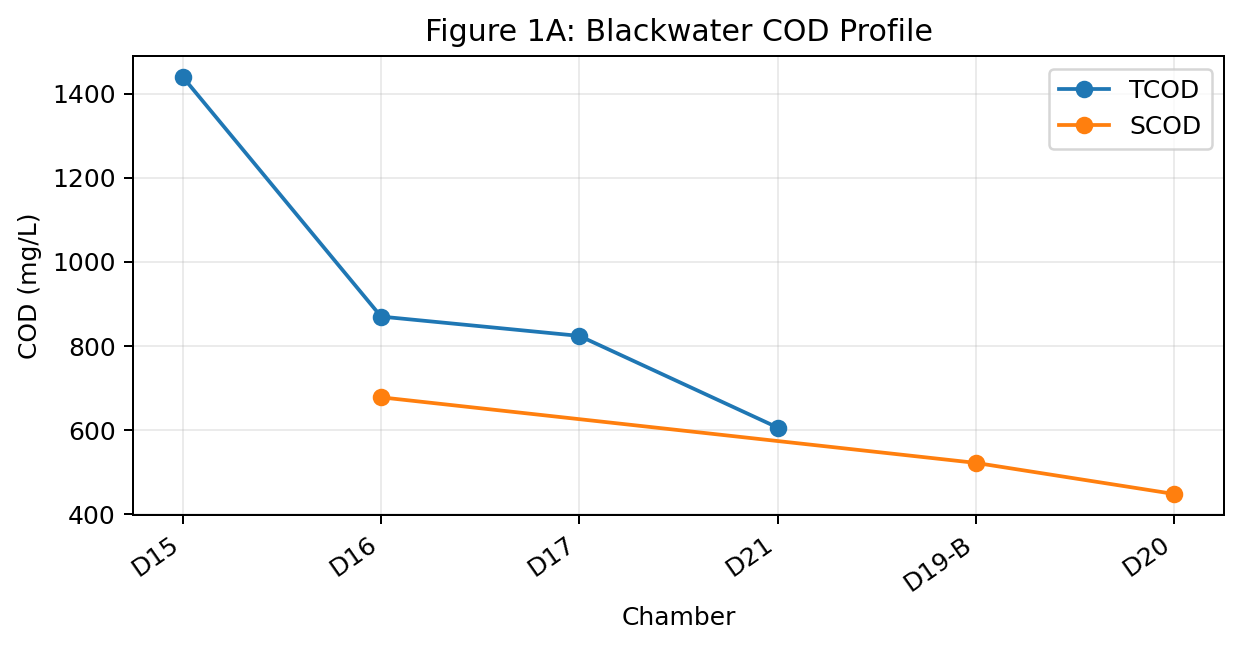
COD is the surrogate for organic matter available for microbial degradation; a progressive decrease between compartments indicates successful substrate utilisation.
| Observation | Interpretation |
|---|---|
| Progressive COD reduction | Active microbial degradation and substrate utilisation |
| COD plateau | Reduced activity, insufficient retention or limited biodegradability |
| COD increase between chambers | Solids resuspension, biomass decay, sludge disturbance or sampling variation |
| High COD throughout | Organic overload or poor treatment progression |
| Minimal COD reduction | Biological underperformance, inhibition or insufficient biomass |
iiOxygen Distribution & Utilisation (ODP / OOUP)aerobic vs anaerobic zoning
The ODP reads DO across sequential compartments (not a single-reactor OUR), giving an operational map of aerobic, oxygen-limited and anaerobic zones. Always read with the CTTP, ORP, pH, nitrogen and biomass.
| DO condition | Zone |
|---|---|
| > 2 mg/L | Aerobic |
| 0.5–2 mg/L | Oxygen-limited |
| < 0.5 mg/L | Anaerobic likely |
| Observation | Interpretation |
|---|---|
| Progressive decline in DO | Active oxygen consumption by microorganisms |
| Stable DO across compartments | Limited biological oxygen demand or reduced activity |
| Sudden increase in DO | Aeration, mixing or polishing stage |
| Persistently high DO with poor COD removal | Possible microbial inhibition or insufficient biomass |
OOUP — Operational Oxygen Utilisation Profile (WESS-specific)
Quantifies the relative DO drawdown between sequential compartments under real operating conditions — a field diagnostic that supports, not replaces, laboratory OUR.
iiiMetabolic State (ORP + DO + pH)dominant pathway
| ORP range | Metabolic state |
|---|---|
| +100 to +400 mV | Aerobic |
| 0 to −100 mV | Anoxic |
| −100 to −250 mV | Anaerobic |
| < −250 mV | Strongly reducing |
| Combined evidence | Interpretation |
|---|---|
| Positive ORP + measurable DO + stable pH | Aerobic biological activity likely |
| Mildly negative ORP + nitrate present/decreasing | Anoxic conditions and possible denitrification |
| Negative ORP + low DO + falling pH | Anaerobic degradation, fermentation or acidogenesis risk |
| Strongly negative ORP + odour/gas | Strongly reducing; sulfide or methanogenic risk |
ivNitrogen transformation & biomass healthN pathway · washout / bulking
Nitrogen transformation (read nitrate/nitrite with ORP + DO)
| Observation | Interpretation |
|---|---|
| Nitrate present + positive ORP | Oxidised nitrogen conditions |
| Elevated nitrite | Incomplete nitrification or unstable nitrogen transformation |
| Decreasing nitrate + mildly negative ORP | Denitrification |
| Nitrate present + strongly reducing ORP | Nitrate present, but active nitrification unlikely under prevailing redox |
Biomass health
| Observation pattern | Interpretation |
|---|---|
| High turbidity + increasing COD | Biomass washout |
| Poor settling + diffuse sludge blanket | Filamentous bulking |
| Excessive foam/scum | EPS overproduction or microbial imbalance |
| Low sludge volume | Biomass loss or poor retention |
| Dense compact sludge | Stable biomass retention |
The HAZOP spine & mitigation catalogue
The same field information, read from the risk side, forms a living HAZOP register. Each of the five treatment compartments is a study node, and v4 adds a sixth — the User-and-Community Interface. For each node the standard guide words (NO, MORE, LESS, REVERSE, PART OF, AS WELL AS, OTHER THAN) are applied to the relevant parameters; a deviation is scored on a 5×5 severity × likelihood matrix, and the score sets the priority of the action exactly as a traffic-light band does.
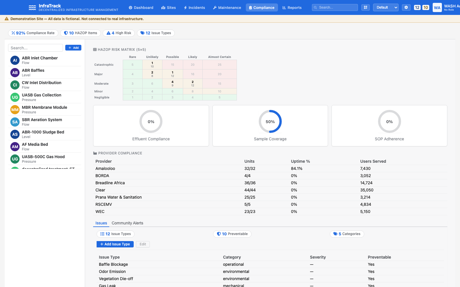
| Node | Parameters | Principal deviations | Protocols |
|---|---|---|---|
| 1 · Primary settling | Flow, level, retention, sludge depth | NO settling; MORE sludge; LESS retention; AS WELL AS foreign objects | 1, 3 |
| 2 · Biological treatment | DO, pH, temperature, biomass activity | NO activity; LESS DO; MORE toxic loading; OTHER THAN expected organisms | 1, 4 |
| 3 · Secondary clarification | Turbidity, SVI, hydraulic loading | MORE solids carryover; LESS settleability; REVERSE (rising sludge) | 1, 3 |
| 4 · Greywater treatment | TDS, turbidity, colour, nutrients | MORE dissolved solids; LESS treatment; AS WELL AS accumulation over cycles | 1, 5 |
| 5 · Disinfection | Cl₂ residual, E. coli, colour, odour | NO disinfectant; LESS pathogen removal; OTHER THAN expected colour/odour | 1, 6 |
| 6 · User & Community | Influent composition, use intensity, stream routing, cleaning inputs | OTHER THAN expected influent (surfactants); AS WELL AS cleaning agents; MORE flush intensity; PART OF / REVERSE greywater diverted | 4, 5 |
The sixth node is a v4 correction and a load-bearing one: reading the register with explicit behaviour classes showed that 29% of entries are behaviour-class, and every one bears on C2 — the process-integrity criterion the cohort fails at every site. Three behaviour-extension deviation classes are scored on the same matrix: cleaning-product chemistry, user behaviour, community practice, with a stated keyword rule so the share is reproducible.
The mitigation catalogue
Every red or amber band carries a defined intervention. The catalogue below is the decision matrix — deviation, its cause, the mitigation, the step that raises it, and whether it is an operating action (OpEx) or a capital/design change (CapEx), and whether it is provider-controllable or driven by household behaviour.
| Deviation | Mitigation | Step | Type |
|---|---|---|---|
| Over-aeration (zoning collapse) | Reduce aeration rate; check baffle integrity between zones | 4, 7 | OpEx · controllable |
| Surfactant / cleaning-product loading | Identify products; community education on WESS-compatible products | 4 | OpEx · behaviour |
| Toxic / low F:M imbalance | Check influent for toxics; increase sludge feed from primary settler | 4 | OpEx · mixed |
| Settling / biological community failure | System reboot (partial/full water replacement) + reseed with live culture | 4, 10 | OpEx · controllable |
| Live culture not on hand | Add live bacterial inoculum to O&M consumables & procurement schedule | 16 | OpEx · controllable |
| Elevated sludge blanket | 40–50%: schedule desludging · >50%: desludge immediately | 6 | OpEx · controllable |
| Dead volume / short-circuiting | Investigate sludge accumulation; assess / modify baffles | 5 | CapEx · controllable |
| Colour / TDS accumulation | Partial reboot (30–50 Pt-Co) or full reboot (>50 Pt-Co / TDS over threshold) | 11–12 | OpEx · controllable |
| Insufficient chlorine | Refill tablets / clear dosing blockage; trace upstream demand | 14 | OpEx · controllable |
| Excessive chlorine | Reduce dosing (by-product & odour risk) | 14 | OpEx · controllable |
| Chlorine recirculating through bio zones | Re-sequence the loop so disinfected water does not re-enter treatment | 14 | CapEx · controllable |
| E. coli elevated with adequate Cl₂ | Particulate shielding → improve upstream treatment / reduce turbidity | 15 | OpEx · controllable |
| Fresh water for reboot not secured | Secure a reboot water supply | 12, 16 | CapEx / logistics |
| Excessive flushing / greywater diversion | Demand management + community practice; engineer tolerance to the behaviour envelope | 12 | Design · behaviour |
| Power supply unreliable | Reliable power (solar / battery / grid) | 16 | CapEx · controllable |
| Structural integrity compromised | Maintenance / repair (leaks, tank condition) | 16 | CapEx · controllable |
The WESS mitigation library
Every recommendation the protocol raises resolves to an entry in a shared mitigation library, each with a stable ID so the same fix is named the same way across sites and its outcomes can be pooled. This is the canonical list — the diagnostics and the lab review both draw from it.
| ID | Mitigation | Typical trigger | Type |
|---|---|---|---|
| M01 | Desludge + sludge-judge cadence (desludge at 50% blanket) | Blanket > 50%; septic COD/TSS climbing | OpEx |
| M02 | System reboot ± reseed with live culture | Biological community failure; inhibitor build-up | OpEx |
| M03 | Increase internal recirculation (anoxic→sedimentation, 3–4× influent) | NO₃ accumulating; denitrification carbon-starved | OpEx |
| M04 | External carbon dose to anoxic (methanol/acetate, ~3 g COD per g NO₃-N) | Internal carbon insufficient for denitrification | OpEx |
| M05 | Chemical-P: alum/PAC jar-test then dose at sedimentation | Phosphorus removal below reuse spec | OpEx / CapEx |
| M06 | Aeration correction (blower / diffuser) | Aerobic DO outside 2–4 mg/L band | OpEx |
| M07 | Re-sequence disinfection loop (chlorinated water out of bio zones) | Recirculation suppressing treatment bacteria | CapEx |
| M08 | GAC polishing stage downstream of disinfection | Colour / organics above reuse spec | CapEx |
| M09 | Install minimum sensor suite to InfraTrack (DO+EC aerobic, turbidity at disinfection) | Sparse / no continuous monitoring | OpEx / CapEx |
| M10 | Rebalance hydraulic distribution across plants | Load imbalance between parallel units | OpEx |
| M11 | Composite sampling + SANAS chain-of-custody | Grab-sample variance; unauditable data | OpEx |
| M12 | TDS reboot SOP (partial drain-down at effluent TDS > 1500 mg/L) | Salt accumulation in the recirculation loop | OpEx |
| M13 | Community education on cleaning products / behaviour envelope | Surfactant load; behaviour-class deviation | OpEx · social |
Priority scoring — which mitigation first
A site can raise a dozen flags; the register is prioritised so the team acts on the right one first. Each candidate mitigation is scored on four axes, each 1–5, and combined:
| Axis | Captures | 1 | 5 |
|---|---|---|---|
| S Severity | Impact of the failure on the seven criteria | Cosmetic; criterion still met | Multiple criteria failing; public-health pathway open |
| C Confidence | How well the data evidence the diagnosis (tier-weighted) | Grab sample only, unconfirmed | SANAS lab + corroborating field tiers |
| I Impact | Expected risk reduction if implemented | Marginal | Brings multiple criteria to On Track / Met |
| E Effort | Cost, time, disruption | Operator action, < 1 day | ≥ 3 months and/or capital |
Priority bands: ≥ 30 Critical (this week / before next visit) · 10–30 High (within 4 weeks) · 3–10 Medium (8–12 weeks) · < 3 Low (document only). A worked, scored register on real lab data is in Part XI, Example 3.
A worked register — Site S001, Visit 1
Each entry is scored on the 5×5 matrix as Likelihood × Consequence; the score sets the priority and drives a linked recommendation. This is a real baseline register from the reporting exemplar — five entries opened at a first visit, each traceable to a field reading in the diagnostics above.
| Entry | Node | Guide word | Deviation | Risk |
|---|---|---|---|---|
| HAZ-001 | Primary settling | NO | No settling after 30 min; SVI not calculable | 12 (3×4) |
| HAZ-002 | Primary settling | MORE | Sludge blanket at 69% of depth; exceeds 50% threshold | 9 (3×3) |
| HAZ-003 | Aerobic polishing | MORE | Persistent dense foam (5 cm) from surfactant loading | 6 (3×2) |
| HAZ-004 | Aerobic polishing | LESS | DO ~47% sat., similar to anaerobic zones; insufficient aeration | 12 (3×4) |
| HAZ-005 | Disinfection | LESS | Free Cl₂ drops to 0.3 mg/L at the toilet interface (below target) | 16 (4×4) |
The linked recommendations
| Action | Priority | Owner | Links |
|---|---|---|---|
| Investigate aeration in the polishing zone; measure air-flow and confirm diffuser condition | High | Provider | HAZ-004 |
| Assess primary settling tank for desludging (blanket 69% > 50%) | High | Provider | HAZ-002 |
| Review chlorine dosing rate; relocate dosing point closer to toilet blocks to hold residual > 0.5 mg/L | High | WESP + Provider | HAZ-005 |
| Develop community awareness material on detergent / cleaning-agent discharge | Medium | WESP team | HAZ-003 |
| Calibrate deployed sensors against laboratory results once available | Medium | L. Naidoo | operational |
| Conduct the residence-time tracer test on anaerobic chamber 1 at Visit 2 | Medium | M. Khan | V2 schedule |
The full register is maintained per site and live in InfraTrack; the recommendations carry a responsible party and a timeline (typically "before the next visit"), and a CapEx recommendation is flagged distinctly from an OpEx one. This is how the assessment ends in a decision and a next step, not a table of numbers.
The data layer & streaming exit
The data layer has two parts. SenseArray is the time-series capture service: a low-cost package built on commodity probes measuring pH, dissolved oxygen, temperature, turbidity, electrical conductivity, TDS and ORP, integrated on a microcontroller platform with local logging and online transmission, installed at the monitored nodes and streaming through a single ingestion endpoint into a central store.
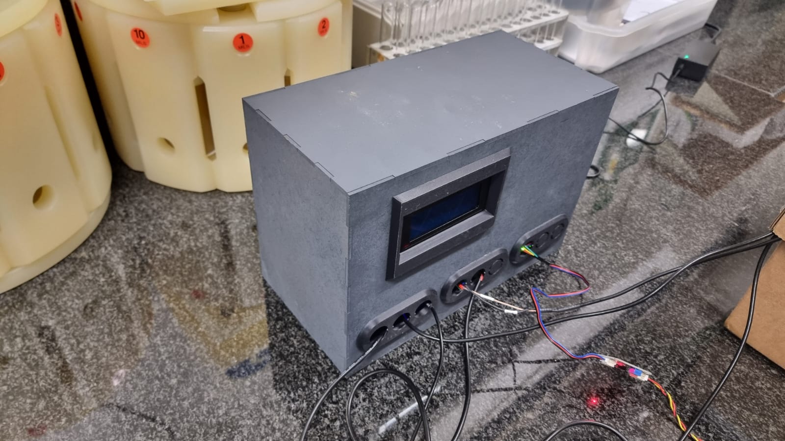
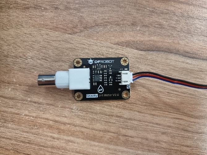
The value of the package is the soft-sensor models on top: multiple-linear-regression models estimate the more expensive compliance parameters — chemical oxygen demand, total nitrogen and phosphate — from the cheap physical measurements, and with drift correction they let that inexpensive, foulable stream substitute for the laboratory between visits. This is exactly the inference the v6 rating consumes, and each physical channel maps to what it can carry:
| Physical channel (measured) | Infers / carries | Confidence |
|---|---|---|
| Turbidity | TSS (physical relationship); COD contribution | Strong — should validate to a high maturity |
| Electrical conductivity, TDS | Ionic load; the TDS proxy between labs | Strong (direct) |
| ORP | Redox / metabolic state; disinfection state | Moderate (context) |
| pH, temperature | Process stability envelope | Direct |
| MLR of the above | COD, total nitrogen, phosphate | Under validation illus. |
| — (no physical proxy) | E. coli / biological count | None — microbial channel, lab-anchored |
Each inference carries a maturity that gates how far it may drive the rating on sensor data alone (the v6 term mk in Part X §B): a strong physical relationship like turbidity→TSS clears the gate early; the MLR estimates of COD, N and P ride between labs only once their prospective validation clears the bar; E. coli never rides the physical stream and stays lab-anchored. The stream is only trusted while it is live and calibrated — a readiness gate checks liveness (expected readings received, in plausible range, tamper-clear), calibration currency (against the last two lab rounds) and drift, and a failure of any drops the node to Provisional rather than passing a stale reading as fresh.
The regression work has reached first results. Models fitted on turbidity, TDS, electrical conductivity and pH return the following Pearson r2 against laboratory analysis, by model degree:
| Model degree (includes constant column) | COD | Total N | P |
|---|---|---|---|
| 1 | 0.735 | 0.533 | 0.983 |
| 2, excluding interaction terms | 0.849 | 0.756 | 0.998 |
| 2, including interaction terms | 0.962 | 0.987 | 1.000 |
These are training fits on a limited dataset, not cross-validated results tested for overfitting, and they will change as site data accumulates. The phosphate column in particular is too good to trust at this sample size and should be read as a sign of overfitting rather than of accuracy. The figures are reported here because the direction is informative — COD and total nitrogen respond strongly to the interaction terms — but no MLR estimate rides the rating on sensor data alone until prospective, cross-validated performance clears the maturity gate.
InfraTrack is the platform on which the record is managed and read: a national status map, the alerts and recommendations as they arise, and the live sensor streams, field observations, laboratory results, HAZOP register and compliance status of every site in one view.
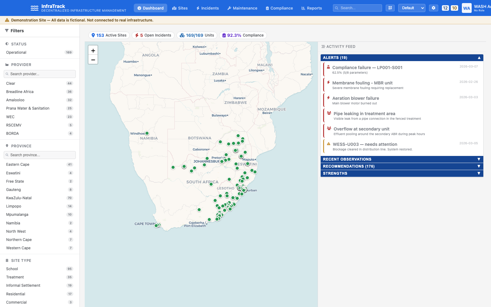
A site is designated de-risked when its subgraph is declared, its HAZOP register is populated, its soft sensors are streaming through SenseArray to InfraTrack showing each monitored node within norms, the laboratory schedule is established, and the O&M staff are trained. From that point the streaming exit makes the v6 live rating possible.
The live rating
The De-Risking Certificate is the financeable artefact, and it has a structural weakness the method's own opening argument exposes: a unit drifts from specification, so a certificate that stamps a time-varying risk at a point in time is decaying from the day it is issued.
Version 6 turns the stream into a live rating on a small ordinal scale the sensor stream maintains and a lender holds as a covenant. One principle runs through every layer — an unknown is a penalised state, not a neutral one.
| Band | State | Condition | Finance consequence |
|---|---|---|---|
| A | De-risked (Live) | All criteria green, stream current and confident, no open high-severity HAZOP node | Full spread benefit (~prime − 3.0 pp) |
| B | Watch | A criterion amber, a leading indicator tripped, or drift detected | Reduced concession; provider notified |
| C | Provisional | Sensor stream degraded/offline, or a lab round overdue | No concession — the site is unobserved |
| D | Breach | A criterion red, or a high-severity HAZOP node realised | Covenant event; remediation window opens |
A fouled or unplugged sensor drops the site to C, and only a confirmatory laboratory round restores A — never the stream simply reading green again. The rating launches on the robustly inferable criteria first (TSS from turbidity, settleability, process state) and treats E. coli and BOD as lab-confirmed inputs that age. The four technical annexes below make it audit-grade.
§AThe rating mathematicsaudit-grade
Compliance and confidence are kept separate: "probably compliant but barely observed" must rate below "probably compliant and confident."
Weights wₖ come from HAZOP severity and the node capacity weights now, the actuarial library later, and are published. Band decision, first match wins: D any criterion confidently red (pₖ<p_red AND cₖ≥c_min) or a realised high-severity node; C confidence below threshold on a material criterion (we do not certify what we cannot see); A S≥S_A AND every material cₖ≥c_min AND no open high-severity node; B everything else. The asymmetry is intentional — failing-but-blind → D; fine-looking-but-blind → C. A bad reading at low confidence routes to C plus a priority verification lab round, never a direct covenant D. Transitions require persistence (n consecutive updates or a CUSUM control-limit breach), with asymmetric hysteresis — easy to fall, hard to rise. Every parameter is a stated, auditable number.
§BThe surrogate-model validation planthe load-bearing dependency
The rating rests on the model inferring the compliance parameters from the cheap stream, so maturity mₖ is earned. For each parameter build a calibrated predictive distribution p(y | x, site, t) — a Bayesian hierarchical (partial-pooling) regression with global coefficients and site random effects, censored-lognormal for E. coli/BOD, with drift terms. A pair is a lab result matched to the concurrent sensor vector (the v4 chain-of-custody fix makes pairs constructible), sampled to span the exceedance region, not just steady-state green. Validate by leave-one-site-out (a new site at V1) and prospective forward-in-time (predict the next lab round), scoring interval coverage and Brier/AUC on P(exceed) near the limit — never in-sample R². The published gate: a criterion may drive an A-band on sensor data alone only when its prospective coverage, exceedance discrimination and paired-evidence count are met; below the gate mₖ is capped low and the criterion stays lab-anchored with a short τ. Expected early outcome: TSS/turbidity clears; E. coli and BOD stay lab-anchored.
§CThe microbial channel in the ratingsee Part V · P8 for full detail
The microbial channel (three tiers, six-strip BioProfile, indices and joint-pattern logic) is documented in full in Part V · P8. Its bearing on the rating: the BioProfile fingerprint decomposes across several criteria (FVI → safety, BFI → fouling, NRFI → nutrients, AEPI → AMR flag), each becoming a pₖ only through lab calibration. Today there is no online microbial stream, so liveness is ≈0 between visits and the criterion is carried by lab-and-BioProfile freshness (short τ), with the laboratory cadence set from τ so a site does not sit at Provisional on public health. Medium-term, the Ramsurran solid-state camera-read indicator supplies a genuine online stream and, once validated, raises mₖ so the microbial criterion can finally ride between visits.
§DThe loan covenanthow the band prices a loan
A margin ratchet — the interest margin a function of the band — prices risk continuously rather than at a cliff (the structure of a sustainability-linked loan); the cliff (event of default) is reserved for sustained failure. The rating-math penalty and the covenant penalty become the same lever: a provider who lets the sensor go dark drops to Provisional and loses the concession that month.
| Band | Margin | Effect |
|---|---|---|
| A Live | prime − 3.0 pp | Full concession |
| B Watch | prime − 1.5 pp | Reduced, under observation |
| C Provisional | prime − 0 pp | No concession — site unobserved |
| D Breach | prime + penalty | Remediation clock; penalty margin during cure |
Operative clauses: reliance & liability (a stated-basis opinion, not a guarantee); data & access covenants (keep the package powered, unobstructed, untampered — closing the gaming loop); remediation & cure (30–60-day window aligned to the between-visit rhythm; restoration needs a confirmatory lab); a standing-service fee (a subscription, borrower-pays, funding recurring telemetry and bi-annual labs — what decouples value from a single loan); independence (the rating entity contractually separate from the platform vendor and provider); and a forward portfolio hook. Fairness point: behaviour-class deviations are 29% of the register, partly outside provider control, so provider-controllable and exogenous drivers are distinguished in the ratchet, or behaviour-class breaches given a longer cure window.
Worked examples
Two field walk-throughs, site identifiers redacted, showing the decision tree end-to-end: real readings resolved into classifications, mitigations, a HAZOP register and an opening rating. Operational thresholds are illustrative; ISO limits are authoritative.
Example 1 — Site α, a household-scale unit at baseline (V1)
A blackwater-line unit (primary settling → anaerobic ×2 → aerobic polishing → disinfection → recirculation). The team runs the observational diagnostics, installs the sensors, and takes the first laboratory round. The readings, by phase:
| Compartment | Blanket ratio | DO (% sat.) | Colour | Foam |
|---|---|---|---|---|
| Primary settling | 61–69% | 2.1 | Black | None |
| Anaerobic 1 | 36–43% | 4.5 | Dark grey | Light scum |
| Anaerobic 2 | 24–28% | 8.2 | Grey-brown | None |
| Aerobic polishing | 10–13% | 46.8 | Light brown | Dense white, 5 cm |
| Disinfection | — | 38.2 | Pale yellow-green | None |
Walking the tree:
- Phase 1 · Settling. The aerobic-polishing zone settles well (SVI 88 mL/g, in-band), but the primary settler shows no measurable settling at 30 min — SVI not calculable. The gate fails; the DSVI/root-cause branch opens, and the cause is immediately visible in Phase 3. → HAZ-001.
- Phase 3 · Sludge. The primary blanket is at 69% of depth — above the 50% critical trigger — thick, paste-like, actively gassing. This sludge overload is why the primary "won't settle": there is no clear water to settle. Decision: desludge now. → HAZ-002. (The settling failure and the sludge reading are one problem seen from two diagnostics — the feedback link in the tree.)
- Phase 4 · Biological. The colour gradient is healthy (black → grey → brown → pale yellow-green = active degradation). But the aerobic polishing DO (46.8% sat.) sits close to the anaerobic zones — insufficient aeration for a polishing stage (→ HAZ-004), and the dense white 5 cm foam flags surfactant loading (→ HAZ-003, a behaviour-class deviation at the User-and-Community node).
- Phase 6 · Disinfection. Free Cl₂ at the toilet interface is 0.3 mg/L, below the 0.5 target — insufficient residual (→ HAZ-005, the highest-scored entry at 16). E. coli sampled for lab confirmation.
The register and its linked actions (the same five entries developed in Part VIII):
| Entry | Deviation | Risk | Action |
|---|---|---|---|
| HAZ-005 | Free Cl₂ 0.3 mg/L at interface | 16 | Review dosing; relocate dosing point closer to blocks |
| HAZ-001 | Primary: no settling / SVI n/a | 12 | Resolve via desludge (HAZ-002); re-test |
| HAZ-004 | Aerobic polishing DO too low | 12 | Investigate aeration; measure air-flow, diffuser |
| HAZ-002 | Primary blanket 69% > 50% | 9 | Desludge before V2 |
| HAZ-003 | Dense foam / surfactant | 6 | Community awareness on cleaning agents |
Opening rating. Process integrity (C2) and effluent quality (C1) are At risk — a red disinfection residual and an under-aerated polishing stage — so on the v6 scale the site would open around B–C: the criteria are not green, and with the sensors only just installed the stream is not yet confident enough to hold A regardless. The three-week action window (desludge, aeration, dosing) is exactly the between-visit remediation the rating's cure logic assumes; a V2 re-test that clears the reds and two confident stream windows are what would carry the site toward A.
Example 2 — Site β, an integrated microbial diagnosis (two lines)
A two-line site (blackwater chambers D15–D21, greywater D22–D27, a septic/sludge node D28). Reading the chamber data through the integrated interpretation (Part VII):
- CTTP: COD declines progressively along the blackwater line → active microbial degradation.
- ODP (DO-lines): the blackwater and greywater lines read as distinct DO paths, rising toward their polishing/aeration ends → oxygen available where expected; the septic node sits low → correct zoning.
- Biomass health: the TSS spike at D17 against a falling COD is the classic turbidity-up-locally signature → a localised biomass washout at that chamber, not a system-wide failure.
- Integrated diagnosis: combined pattern = healthy oxidative activity along both lines with one washout point. FMHI: most indicators green, biomass/TSS amber at D17 → compartment band AMBER localised to D17 → increase monitoring there, check the D17 hydraulics/settling, and confirm with the next lab round. No red, no system intervention.
Example 3 — Site γ, reading a laboratory report into mitigations
A 63-household site running three parallel biological plants (influent → anaerobic → sedimentation → aerobic → anoxic → 2nd sedimentation → disinfection), treated water reused for flushing only. Five accredited (SANAS) laboratory reports were reviewed. The final-effluent report is read parameter by parameter — each value against expectation, then to a mitigation from the library:
| Parameter | Value | Reading & decision |
|---|---|---|
| E. coli | 1 CFU/100 mL | Disinfection working — down from 13 000 (≈4-log). Meets the health target. |
| BOD₅ | 6 mg/L | 97% removal (from 213). Well within ISO Cat A (≤10). |
| TSS | 8.0 mg/L | 69% removal (from 26). Within Cat A (≤10). |
| COD | 66.4 mg/L | Within Cat B (≤150) but close to the ~75 discharge ceiling — thin margin against load shocks. |
| NO₃-N | 47.3 mg/L | Nitrification complete but denitrification is not occurring — the anoxic stage is not delivering. → M03/M04 |
| NO₂-N | 4.17 mg/L | Non-trivial — nitrite-oxidisers lagging ammonia-oxidisers; track visit-to-visit. |
| Total P | 9.78 mg/L | Only ~67% removal; no chemical-P stage. Blocks any <5 mg/L reuse spec. → M05 |
| TDS | 1 234 mg/L | High and climbing as the reuse loop concentrates salts. Set a reboot rule at >1500. → M12 |
| True colour | 129 Pt-Co | Acceptable for flush; visually noticeable. GAC polishing if reuse extends. → M08 |
| DO | 5.27 mg/L | Confirms the aerobic chamber is functioning. |
The septic chamber tells a second story: COD climbed 1 657 → 5 691 and TSS 42 → 2 544 over two months with no desludge cadence — the single highest-severity finding. Consolidating every flag through the priority scoring (S×C×I/E) gives a register that acts on the right thing first:
| Mitigation | S | C | I | E | Priority |
|---|---|---|---|---|---|
| M01 Desludge septic + sludge-judge cadence | 5 | 5 | 5 | 1 | 125 Critical |
| M11 Composite sampling + SANAS chain-of-custody | 3 | 5 | 3 | 1 | 45 Critical |
| M10 Rebalance load across the three plants | 4 | 4 | 4 | 2 | 32 Critical |
| M12 TDS reboot SOP (> 1500) | 2 | 4 | 3 | 1 | 24 High |
| M09 Minimum sensor suite to InfraTrack | 3 | 5 | 4 | 3 | 20 High |
| M03/M04 Recirculation audit + carbon on standby | 3 | 4 | 4 | 3 | 16 High |
| M05 Alum/PAC jar-test for phosphorus | 2 | 4 | 3 | 3 | 8 Medium |
The scoring corroborates the engineering judgement — desludge and load-rebalance surface first — and additionally promotes the sampling-protocol fix (M11) that a narrative read under-weights: the January-to-March influent ammonium varied 60× on the same plant, which is more plausibly grab-sample variance than a real influent change, and until the data are auditable every downstream diagnosis inherits that uncertainty.
Cost & financial de-risking
Before the numbers, the approach. Financial de-risking converts the engineering record this protocol produces into a price: a lender who can see an independent operating record prices the loan against evidence rather than against uncertainty, and the spread falls. The mechanism has three parties. The technology provider sources the finance — it is the provider who borrows, from a commercial bank, to manufacture and deploy units at scale, and the provider who carries the interest cost that de-risking reduces. The de-risking engagement is paid for separately and in advance of the loan: under the WESP De-Risking Fund the per-site cost is co-funded 50/50 between the fund (seeded by the Water Research Commission, financial institutions and corporate social investment) and the provider, keeping the provider's incentive aligned with the outcome. The lender pays nothing, and receives the certificate — in v6, the live rating held as a covenant — as the independent record it otherwise lacks. The municipality or site owner enters not as a financier of the de-risking but as the payer for the sanitation service whose reliability the whole arrangement secures.
Within that structure, a full engagement is of the order of R 175,000 per site.
| Cost item | Amount |
|---|---|
| Engineering personnel — three visits, field and analysis | R 78,000 |
| Laboratory analysis — settleability, sludge, microbial, compliance | R 40,000 |
| Soft-sensor package, installation and first-year telemetry | R 30,000 |
| Travel and site logistics — three visits | R 15,000 |
| Field consumables and test kits | R 7,000 |
| Reporting and certification | R 5,000 |
| Total per site | R 175,000 |
Under the WESP De-Risking Fund the cost is met 50/50, so the provider carries about R 87,500. Under v6 the telemetry and laboratory lines become recurring — the standing-service fee — rather than one-off.
The bankability case
On an illustrative R 3,000,000 loan over five years, a three-percentage-point reduction in spread saves roughly R 266,000 in interest over the term:
| At prime (11.5%) | At prime − 3 pp (8.5%) | |
|---|---|---|
| Monthly repayment (R 3.0m, 5 yr) | R 65,978 | R 61,550 |
| Total interest over the term | R 958,669 | R 692,976 |
| Interest saving | — | R 265,694 |
| Net benefit to the provider | — | ≈ R 178,000 |
Net benefit reaches zero at a break-even spread reduction of about one percentage point for this loan, rising as the loan shrinks. The one input the field programme cannot supply — the spread a certificate actually earns — is a stated objective of the commercial-bank engagement, which in v6 widens to fixing the whole ratchet and covenant structure. Each de-risked site is also a reference case for the provider's next application, and the recurring rating fee is a standing revenue line rather than a cost amortised against one facility.
Bankability at portfolio scale: ten sites
The single-site table understates the case, because the lender's real question is about a deployment, not a unit. For an illustrative programme of ten sites, each financed as above:
| Portfolio line (10 sites, illustrative) | Amount |
|---|---|
| Loan book (10 × R 3.0m, 5 yr) | R 30,000,000 |
| Interest saving at a 3 pp spread reduction, over the term | ≈ R 2,660,000 |
| De-risking cost (10 × R 175,000, before the 50/50 co-funding) | R 1,750,000 |
| Provider's share under the Fund (10 × R 87,500) | R 875,000 |
| Net benefit to the provider across the portfolio | ≈ R 1,785,000 |
Three things change at this scale that no single site shows. The evidence compounds: ten monitored sites give the lender a distribution, not an anecdote, so the priced risk falls further than the per-site arithmetic suggests. The fixed costs dilute: the engineering team, the laboratory relationship and the data platform are stood up once and amortise across the book, so the marginal site costs less than the first. And the portfolio becomes the covenant: under v6 the lender holds not ten certificates but one live view of a rated fleet, which is the instrument a development financier or a securitising bank can actually work with. Bankability, for a ten-site programme, means the de-risking pays for itself out of the interest saving alone, before any value is placed on the reference cases, the standing-service revenue, or the faster approval of the next ten.
Circular-economy context
The circular-economy framing held up in the field and is carried unchanged from v3 — on the reference model it is the residuals-and-recovery lane. Open it if you need it.
XIIWESS as circular-economy infrastructurerecirculation · nutrients · sludge · energy · policy
Water recirculation. The unit recovers treated water for flushing and reuse, closing the loop at the point of generation.
Nutrient recovery. Nitrogen and phosphorus concentrated by the train can be recovered rather than discharged — the nutrient-recovery node, fed by the nitrogen-removal read.
Sludge valorisation. Solids characterised by the sludge-profile diagnostic can be valorised as biochar or compost, turning a desludging cost into a product.
Energy balance. The community reference site runs entirely on solar power; the protocol assesses the energy balance as part of operational sustainability.
Policy positioning. The method sits within the revised ISO 30500 (2025), SANS 241 and the draft model by-laws defining WESS as a non-sewered sanitation category permitted to treat and reuse water on site.
Team & trajectory
The programme is delivered by a small core team, each member holding one axis, so the eight diagnostics are the field expression of seven specialisms. In the KwaZulu-Natal cluster the team is joined by two eThekwini Municipality trainee engineers.
- Prof Randhir Rawatlal — programme lead; the de-risking framework, the decision model, and the financial de-risking with the commercial-bank partner.
- Dr Russ Ngosa — engineering diagnostics and re-engineering; the HAZOP methodology and simulator/model validation.
- Leesan Naidoo — low-cost sensing and the continuous-monitoring exit; the soft-sensor array, drift correction, and the v6 surrogate-validation plan.
- Muhammad Ameen Khan — process modelling and residence-time analysis; the WESS process and population-balance models and the tracer studies.
- Gloseje Khanyinda — greywater characterisation and treatment sequencing.
- Mxolisi Vundla — sludge accumulation, settleability and valorisation.
- Dr Riona Indhur — microbial functional profiling; the WESScheck BioProfile field screen.
The framework is exercised and stable; what remains is depth of coverage — the sensor-streaming final visits, the Lilliput trio's first visits in Q3 2026, and the spread a certificate earns confirmed against a real lender. Phase 2 extends the framework to twenty further sites with train-the-trainer coursework for municipal engineers (CPD through the Water Institute of Southern Africa), transferring the capacity to de-risk a site to the Water Services Authorities that will own these installations. The Centre's independence rests on holding no equity and manufacturing no technology; the rating log is portable and third-party auditable.
Across the roughly eighteen months of this work, the programme's evidence base was built visit by visit at real installations. We thank the WESS technology providers — Enviroloo, Prana Aquonic, WEC and Lilliput — for their openness to independent assessment and their willingness to act on the findings; a de-risking method can only be field-tested on units that someone has built and is prepared to have measured.
Record of site visits
The programme is not a desk exercise. This is the field record — every site engaged, when, and what came out of it — kept both as an evidence trail and to show the funders the volume of work behind the method. Site and provider names are replaced by consistent hash codes (the same site always carries the same code); the document links open the underlying reports on the local drive.
Reach to date: 9 sites · 4 technology providers (P-B672 · P-99B4 · P-BEF5 · P-B320) · 2 provinces · 5 formal baseline assessments + 1 mid-point review + 3 onboardings + a 5-report accredited-lab review · 24 HAZOP entries and 49 engineering recommendations, each traceable to a field measurement · field visits Jan–Jul 2026, within the ~18-month programme.
| Site | Provider | Region | Visit(s) & date | HAZOPs | Recs | Outcome | Report |
|---|---|---|---|---|---|---|---|
| S-DC33 | P-B672 | KZN | Baseline · 2026-02-06 + Mid-point · 2026-03-20 | 6 | 17 | At-risk process status at baseline; sludge overload, under-aeration and low chlorine residual actioned; returned for a mid-point review. | V1 report · V2 report · Field report |
| S-1B42 | P-BEF5 | KZN | Baseline · 2026-02-25 | 4 | 6 | Baseline assessment; process integrity at risk; recommendations issued. | Field report |
| S-0E31 | P-BEF5 | KZN | Baseline · 2026-02-09 | 2 | 4 | Baseline assessment; field record and photographs captured. | Anonymised report |
| S-4783 | P-BEF5 | Gauteng | Baseline · 2026-02-06 | 7 | 11 | 620-household community system — the most HAZOP entries of any site, the community-scale complexity a desk review does not surface. | Field report |
| S-F14E | P-B320 | KZN | Baseline + greywater · 2026-04-14 | 5 | 11 | Two-line site (blackwater + greywater); integrated microbial diagnostics and the paired greywater evaluation; microbial review and mitigations issued. | Microbial review |
| S-2D8B | P-BEF5 | — | Lab review — 5 accredited reports · 2026-01-14 / 2026-03-12 | — | 8 | 63-household site (3 Aquonic plants); five SANAS-accredited laboratory reports reviewed — denitrification failure and septic accumulation the critical findings; 8-item scored mitigation register. | Lab review & mitigations · Aquatico effluent report |
| S-2785 | P-99B4 | KZN | Onboarding · 2026-05-19 | — | — | Onboarded for first-visit assessment. | Onboarding report |
| S-3792 | P-99B4 | KZN | Onboarding · 2026-05-19 | — | — | Onboarded for first-visit assessment. | Onboarding report |
| S-7474 | P-99B4 | KZN | Onboarding · 2026-05-19 | — | — | Onboarded; first site report issued. | Site report · Onboarding report |
file:// references to documents on the WASH R&D drive — they open when this page is viewed locally (or from the Word edition on the same machine); a shared web copy cannot open a local file. This appendix is a live index, not the reports themselves.The site report template
Every visit ends in a report, and every report follows one template, so a provider, a municipality or a lender reading their third report can navigate it as fast as their first. The template below is the structure every site report in the Appendix A record follows; on the monitoring platform the same template is generated directly from the visit data.
| Section | Contents | Source in this protocol |
|---|---|---|
| 1 · Site identification | Site and provider (coded where circulated), configuration against the reference model, reuse destination, visit number and date, personnel | Part II declaration; Part IV visit plan |
| 2 · Data status | The single-round caveat where it applies; sample codes against the chain-of-custody legend; any quality flags | Part VII gates |
| 3 · Executive summary | Opens with what the data shows working, then the excursions — each finding stated once, with its measurement, mechanism and action; classifications carry their confidence grade (Confirmed / Provisional / Re-test required) | Part V diagnostics; the reporting style guide |
| 4 · Compartment classifications | The green/amber/red status per compartment with the measured values and the branch taken in the decision tree | Parts III & V |
| 5 · Laboratory results | Parameter table against the destination's compliance bands; each excursion mapped to a mitigation | Part VII interpretation guide |
| 6 · Completion criteria roll-up | C1–C7 with status and evidence base; the social-framework rung alongside C4/C6 | Part VI |
| 7 · HAZOP register update | Entries opened, progressed and closed this visit, with guide words and owners | Part VIII spine |
| 8 · Mitigations & actions | The priority-scored mitigation list from the library, each with its trigger measurement and its owner | Part VIII catalogue |
| 9 · Next visit | What will be measured to confirm each provisional finding and each mitigation's effect; sensor and rating status where installed | Parts IV, IX & X |
The template is deliberately symmetrical with the protocol: a reader can put any report section beside the part of this document that produced it and see the method behind the finding — which is what makes the reports auditable, and what makes the protocol trainable.